flowchart TD
    A["Prior admissions ≥ 2?"] -->|Yes| B["Has heart failure?"]
    A -->|No| C["Age ≥ 75?"]
    B -->|Yes| D["High risk<br/>~62% readmit"]
    B -->|No| E["Moderate risk<br/>~34% readmit"]
    C -->|Yes| F["Moderate risk<br/>~28% readmit"]
    C -->|No| G["Low risk<br/>~9% readmit"]
    style D fill:#e8736a,color:#fff
    style E fill:#f4c06a
    style F fill:#f4c06a
    style G fill:#7fc08a,color:#fff
13 Decision Trees, Random Forests, and Gradient Boosting
Of all the machine learning methods covered here, tree-based methods tend to be adopted fastest by clinicians. One reason is that they mirror how clinical reasoning works. A doctor triaging chest pain mentally runs through a series of questions (“Is the troponin elevated? Are there ECG changes? Is the patient over 65?”), and each answer narrows down the likely diagnosis. That branching logic is a decision tree. This chapter starts from that intuition and builds up to the methods that win most clinical prediction competitions on tabular data: random forests and gradient boosting, which combine hundreds of trees into a single, far more accurate model.
Why invest in these methods rather than stopping at logistic regression? Because they automatically capture two things that are pervasive in medicine and awkward for standard regression: non-linear effects (e.g., risk that rises sharply only past a threshold) and interactions (e.g., a lab value that matters only in diabetic patients). You do not have to specify these by hand — the trees discover them. The price is interpretability, which is why the chapter spends time on how to read a tree and how to inspect variable importance.
13.1 Decision Trees
A decision tree is perhaps the most intuitive machine learning model. It makes predictions by asking a series of yes/no questions about the input features, splitting the data at each step into increasingly homogeneous groups. Each node is a test on a single feature (e.g., is age <= 30?), and branches are the possible answers (e.g., yes/no). The leaves at the bottom of the tree represent the final prediction (e.g., high risk or low risk). The resulting structure looks like an inverted tree — hence the name.
Why start with decision trees? Decision trees (also called classification and regression trees (CART)) are the foundation for all tree-based methods we will cover in this chapter, which rely on ensembling many trees. But a single tree is also valuable in its own right for clinical work: it produces a rule you can literally read off and apply at the bedside without a computer, and it handles a mix of continuous and categorical predictors, missing values, and interactions with no special preprocessing. When you need a model that a clinical team will actually trust and use, a small decision tree is often a practical choice. Figure 13.1 shows the kind of transparent rule a tree produces.
13.1.1 How Trees Split
The algorithm works top-down, greedily selecting the best split at each node. “Greedy” means it takes the single best step available right now without looking ahead — like a clinician ordering the one test that best separates the likely diagnoses at this moment, then reassessing. Concretely:
- Consider every feature and every possible split point. For a continuous variable like age, the tree tries every threshold (“age < 60?”, “age < 61?”, …); for a binary variable like has diabetes, there is only one possible split. So at the very first node the algorithm might evaluate thousands of candidate questions.
- Score each candidate split by how much it improves the “purity” of the two resulting groups. A split is good if it sends mostly-readmitted patients down one branch and mostly-not-readmitted patients down the other. “Purity” is just a number measuring how one-sided a group is (defined precisely in the next section).
- Choose the single split that improves purity the most, and use it to divide the patients into two child nodes.
- Repeat recursively on each child node — each becomes a new little problem with its own best question — until a stopping criterion is met: the node is too small to split further (
minsplit), the tree has reached its maximum allowed depth (maxdepth), or no remaining split improves purity enough to be worthwhile.
A worked picture: at the root, the algorithm might find that “prior admissions ≥ 2?” best separates readmitted from non-readmitted patients. Among the patients who answered “yes,” it then searches again and might pick “has heart failure?”; among those who answered “no,” it might instead pick “age ≥ 75?”. Different branches can ask about different variables — this is precisely how trees capture interactions automatically.
13.1.2 Splitting Criteria
“Purity” needs to be turned into a number the computer can compare. Impurity is simply a score for how mixed a group of patients is: it is 0 when everyone in the group has the same outcome (all readmitted, or all not) and largest when the group is a 50/50 coin-flip. A split is judged good when it produces child groups that are purer (lower impurity) than the parent. Two formulas are used to measure this; do not be put off by the notation — each is a short, self-contained expression that you will not need to evaluate by hand.
In the formulas below, imagine a group of patients in which a fraction \(p_1\) have outcome 1 (readmitted), \(p_2\) have outcome 2, and so on, across \(K\) possible outcomes. For the binary readmission example there are just two: \(p_{\text{yes}}\) and \(p_{\text{no}} = 1 - p_{\text{yes}}\).
Gini impurity — the chance two randomly drawn patients from the group have different outcomes:
\[G = \sum_{k=1}^{K} p_k (1 - p_k) = 1 - \sum_{k=1}^{K} p_k^2\]
Read it as: each outcome contributes a term \(p_k(1 - p_k)\) — largest when that outcome is a coin-flip — and summing these measures how “spread out” the group is across outcomes. Gini is 0 when a node is pure (all one class) and maximised when classes are equally mixed. For a binary problem the maximum is 0.5, reached at \(p = 0.5\).
Worked example. A node of 100 patients with 30 readmitted and 70 not has \(p_{\text{yes}} = 0.30\), \(p_{\text{no}} = 0.70\), so \(G = 1 - (0.30^2 + 0.70^2) = 1 - (0.09 + 0.49) = 0.42\) — fairly impure. If a split sends 40 patients to a child node that is 35 readmitted / 5 not (\(p = 0.875\)), that child has \(G = 1 - (0.875^2 + 0.125^2) = 0.22\) — much purer. The tree favours splits that drive these child Gini values down.
Entropy (information gain) — an alternative impurity measure borrowed from information theory:
\[H = -\sum_{k=1}^{K} p_k \log_2(p_k)\]
It behaves almost identically to Gini: 0 when the node is pure, and maximised (at \(\log_2 K\)) when outcomes are evenly split. The reduction in entropy achieved by a split is called the information gain.
In practice, Gini and entropy produce very similar trees, so the choice rarely matters. Gini is the default in most implementations because it is slightly faster to compute (no logarithm). You do not need to compute these by hand — the software does it for every candidate split. The reason to understand them is to know what the tree is optimising: at each step it is hunting for the question that most cleanly separates the outcomes.
For regression trees (continuous outcomes, e.g. predicting length of stay), there are no classes to count, so impurity is instead the variance within the node. A split is good when it produces child nodes whose values are tightly clustered — equivalently, when it gives the largest reduction in residual sum of squares.
13.1.3 Clinical Example: Hospital Readmission
Let us build a decision tree to predict 30-day hospital readmission — a common quality metric tied to reimbursement penalties in the United States.
Code
# Decision trees are built with the rpart package; rpart.plot draws them.
# tidyverse provides tibble() and the data-handling verbs used below.
library(tidyverse)
library(rpart)
library(rpart.plot)

# Simulate hospital readmission data
set.seed(42)
n <- 1000

readmit_data <- tibble(
  age = rnorm(n, 68, 12),
  length_of_stay = rpois(n, 5) + 1,
  num_comorbidities = rpois(n, 3),
  prior_admissions = rpois(n, 1),
  discharge_hemoglobin = rnorm(n, 11, 2),
  discharge_creatinine = rlnorm(n, 0.2, 0.5),
  has_diabetes = rbinom(n, 1, 0.35),
  has_chf = rbinom(n, 1, 0.25),
  readmitted = factor(
    rbinom(
      n,
      1,
      plogis(
        -3.5 +
          0.05 * (age - 68) +
          0.7 * prior_admissions +
          0.25 * num_comorbidities +
          1.3 * has_chf -
          0.25 * (discharge_hemoglobin - 11)
      )
    ),
    labels = c("No", "Yes")
  )
)

cat("Readmission rate:", round(mean(readmit_data$readmitted == "Yes"), 3), "\n")
cat("N =", nrow(readmit_data), "\n")
Code
# Fit a decision tree
tree_model <- rpart(
  readmitted ~ age +
    length_of_stay +
    num_comorbidities +
    prior_admissions +
    discharge_hemoglobin +
    discharge_creatinine +
    has_diabetes +
    has_chf,
  data = readmit_data,
  method = "class",
  control = rpart.control(cp = 0.01, maxdepth = 5, minsplit = 20)
)

# Visualize
rpart.plot(
  tree_model,
  type = 4,
  extra = 106,
  under = TRUE,
  box.palette = "RdYlGn",
  roundint = FALSE,
  main = "Decision Tree: 30-Day Readmission"
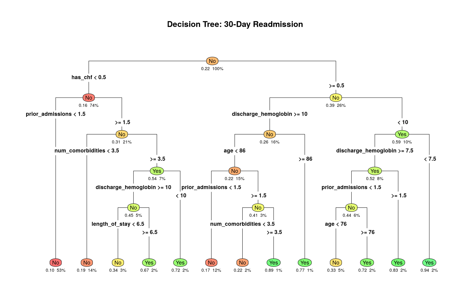
)
Code
import numpy as np
import pandas as pd
from sklearn.tree import DecisionTreeClassifier, plot_tree
from sklearn.model_selection import cross_val_score, StratifiedKFold
import matplotlib.pyplot as plt

np.random.seed(42)
n = 1000

df = pd.DataFrame({
    'age': np.random.normal(68, 12, n),
    'length_of_stay': np.random.poisson(5, n) + 1,
    'num_comorbidities': np.random.poisson(3, n),
    'prior_admissions': np.random.poisson(1, n),
    'discharge_hemoglobin': np.random.normal(11, 2, n),
    'discharge_creatinine': np.random.lognormal(0.2, 0.5, n),
    'has_diabetes': np.random.binomial(1, 0.35, n),
    'has_chf': np.random.binomial(1, 0.25, n)
})
# Outcome depends on the predictors (mirrors the R simulation)
logit = (-3.5
         + 0.05 * (df['age'] - 68)
         + 0.70 * df['prior_admissions']
         + 0.25 * df['num_comorbidities']
         + 1.30 * df['has_chf']
         - 0.25 * (df['discharge_hemoglobin'] - 11))
y = np.random.binomial(1, 1 / (1 + np.exp(-logit)))

feature_names = list(df.columns)

# Fit decision tree
tree = DecisionTreeClassifier(max_depth=5, min_samples_split=20,
                               min_samples_leaf=10, random_state=42)
tree.fit(df, y)

fig, ax = plt.subplots(figsize=(16, 8))
plot_tree(tree, feature_names=feature_names, class_names=['No', 'Yes'],
          filled=True, rounded=True, ax=ax, fontsize=8, max_depth=3)
ax.set_title("Decision Tree: 30-Day Readmission")
plt.tight_layout()
plt.show()
DecisionTreeClassifier(max_depth=5, min_samples_leaf=10, min_samples_split=20,
random_state=42)In a Jupyter environment, please rerun this cell to show the HTML representation or trust the notebook. On GitHub, the HTML representation is unable to render, please try loading this page with nbviewer.org.
Parameters
Fitted attributes
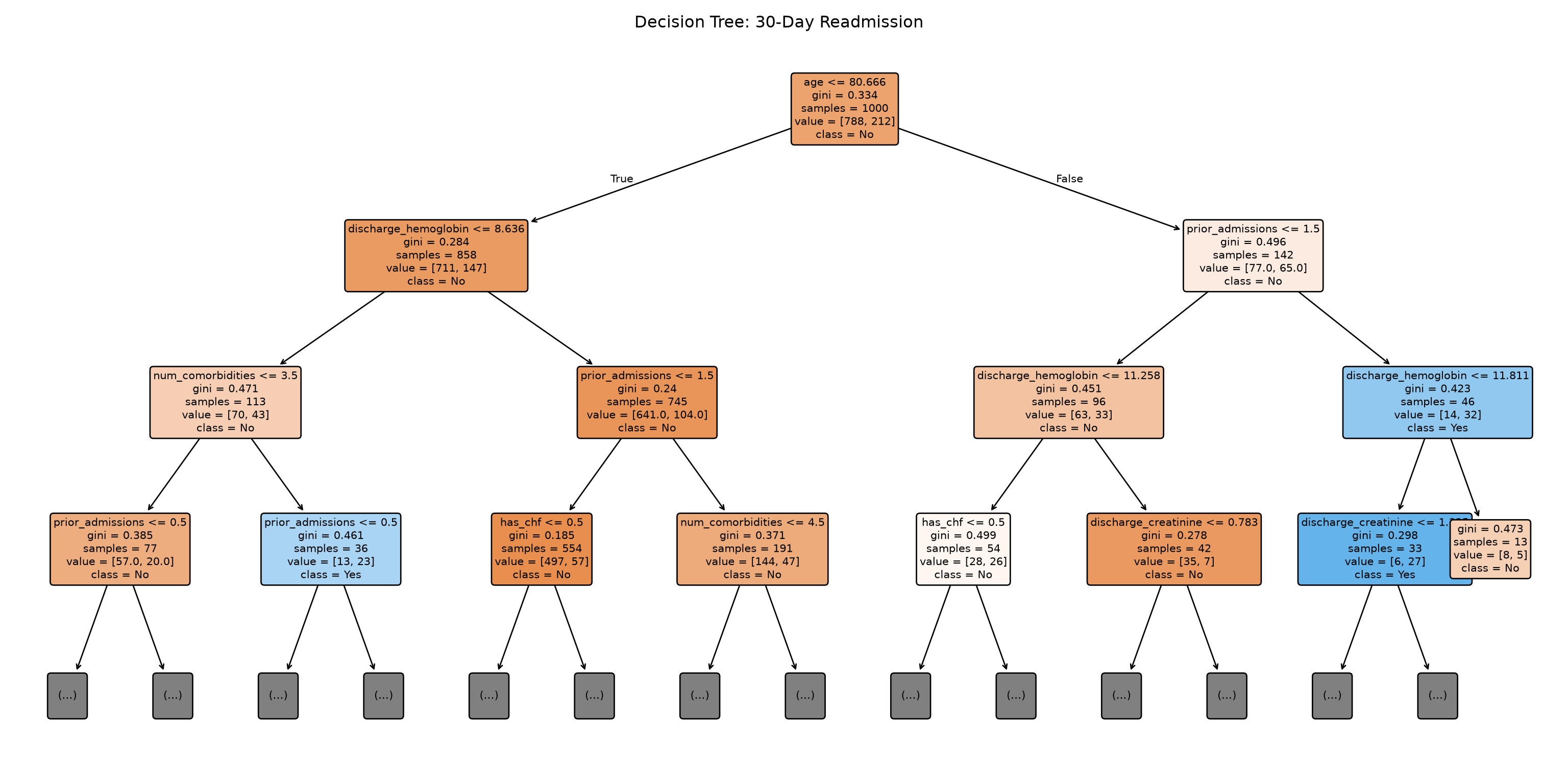
A classification tree for 30-day readmission (first three levels shown). Read it top-down, following each yes/no answer to a leaf.
13.1.4 Reading a Decision Tree
Each node in the tree displays:
- The splitting rule (e.g., “age >= 72”)
- The predicted class (the majority class in that node)
- The class probabilities (e.g. 0.34 readmitted / 0.66 not)
- The percentage of observations that reach this node
The root is simply the single box at the very top of the tree — the first question, asked of every patient before any splitting. Do not be surprised if the root node is labelled “No”: the label on any node (root included) is just the majority outcome among the patients sitting in it, and since most patients are not readmitted, the whole-cohort majority — and therefore the root’s label — is “No”. The label becomes informative only further down, once splits have concentrated the higher-risk patients into particular leaves.
To classify a new patient, start at the root and follow the branches based on the patient’s feature values until you reach a terminal node (leaf). The prediction is the majority class of that leaf, and the leaf’s class probability is the patient’s estimated risk.
Worked example. Suppose a 78-year-old patient has had no prior admissions and no heart failure. Starting at the root of Figure 13.1, “prior admissions ≥ 2?” is No, so we go right to “age ≥ 75?”, which is Yes, landing in the moderate risk leaf (~28% readmission risk). A different patient with three prior admissions and heart failure follows the left branches into the high risk leaf (~62%). Notice two clinically useful properties: the prediction is reached by at most a handful of questions, and you can explain exactly why any patient received their risk estimate — a transparency that “black box” models cannot offer. The flip side is that a single tree’s boundaries are coarse (everyone in a leaf gets the same risk) and can shift noticeably if the data change slightly, which is the motivation for the ensemble methods later in this chapter.
13.1.5 Pruning: Controlling Tree Complexity
Why pruning matters. A tree left to grow without limits will keep asking questions until each leaf contains just one or two patients — effectively building a private rule for every individual in the training set. It will look perfect on the data it was built from and then fail badly on new patients, because it has memorised noise (one patient’s quirky lab value) instead of learning generalisable patterns. This is overfitting, and for a clinical tool it is dangerous: a model that boasts 99% accuracy in development but collapses in the next clinic is worse than no model, because people trusted it.
Pruning is the cure: it deliberately cuts the tree back to a smaller, simpler set of rules that capture the real signal and ignore the noise. A pruned tree usually performs slightly worse on the training data but better on new patients — which is the only performance that matters. Think of it as the bias–variance tradeoff (from the previous chapter) made tangible: a few extra mistakes in development buy a large gain in reliability. The goal is the smallest tree whose performance is statistically indistinguishable from the bigger one.
Two strategies:
Pre-pruning (early stopping): Set constraints before growing the tree — maximum depth, minimum samples per leaf, minimum information gain to split. Simple but can stop too early.
Post-pruning (cost-complexity pruning): Grow a full tree, then cut back the branches that barely help. In R’s
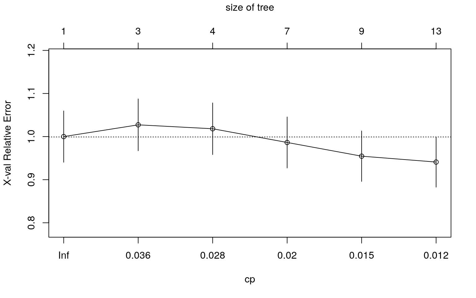
rpart, how aggressively you cut is governed by a single knob, the complexity parameter (cp): it is the minimum improvement a split must deliver to be kept, expressed as a fraction of the tree’s overall error. A largecpdemands that every split earn its keep, so the tree stays small; a smallcplets the tree grow bushy. Rather than guess a value, we let cross-validation choose it: we try a range ofcpvalues, see which gives the best error on held-out data, and prune to that one (shown in the code below).
Code
Code
# Prune to optimal cp
optimal_cp <- tree_model$cptable[
  which.min(tree_model$cptable[, "xerror"]),
  "CP"
]
pruned_tree <- prune(tree_model, cp = optimal_cp)

cat("Optimal cp:", round(optimal_cp, 4), "\n")
cat(
  "Number of terminal nodes (full):",
  sum(tree_model$frame$var == "<leaf>"),
  "\n"
)
cat(
  "Number of terminal nodes (pruned):",
  sum(pruned_tree$frame$var == "<leaf>"),
  "\n"
)| CP | nsplit | rel error | xerror | xstd |
|---|---|---|---|---|
| 0.0409 | 0 | 1.0000 | 1.0000 | 0.0595 |
| 0.0318 | 2 | 0.9182 | 1.0273 | 0.0601 |
| 0.0242 | 3 | 0.8864 | 1.0182 | 0.0599 |
| 0.0159 | 6 | 0.8136 | 0.9864 | 0.0592 |
| 0.0136 | 8 | 0.7818 | 0.9545 | 0.0585 |
| 0.0100 | 12 | 0.7091 | 0.9409 | 0.0582 |
Cross-validation error as a function of the complexity parameter. The optimal cp minimizes the cross-validated error.
Optimal cp: 0.01
Number of terminal nodes (full): 13
Number of terminal nodes (pruned): 13
Code
from sklearn.tree import DecisionTreeClassifier
from sklearn.model_selection import cross_val_score
import numpy as np

# Compare trees of different depths
depths = [2, 3, 5, 7, 10, 15, None]
cv = StratifiedKFold(n_splits=5, shuffle=True, random_state=42)

results = []
for d in depths:
    t = DecisionTreeClassifier(max_depth=d, random_state=42)
    scores = cross_val_score(t, df, y, cv=cv, scoring='roc_auc')
    depth_label = str(d) if d is not None else "None (full)"
    results.append({'max_depth': depth_label,
                    'mean_auc': scores.mean(),
                    'std_auc': scores.std()})
print(f"max_depth={depth_label:>6s}: AUC = {scores.mean():.3f} (+/- {scores.std():.3f})")What the code is showing. Both versions answer the same question — how big should the tree be? — by measuring performance on held-out data rather than the training data:
- The R version uses cost-complexity pruning.
printcp()prints a table where each row is a candidate tree size, and the key column isxerror(the cross-validated error). As the tree grows,xerrorfirst falls (the tree is learning real structure) and then rises again (it has started memorising noise).plotcp()shows this as a U-shape. The code picks the complexity parametercpat the bottom of the U and prunes to it; the final two lines print how many leaves the full tree had versus the smaller pruned tree — you should see the pruned tree is considerably smaller. - The Python version makes the same point more directly by sweeping
max_depthfrom 2 up to “no limit” and printing the cross-validated AUC for each. Reading down the list, AUC climbs, peaks at a modest depth, then stops improving (or worsens) as the tree gets deeper — and the script reports the depth that won. The deepest tree is not the best.
The shared lesson: deeper is not better. The right-sized tree is the one that does best on patients it has never seen, and cross-validation is how you find it.
13.2 Why Single Trees Are Unstable
Decision trees have a critical weakness: high variance. Small changes in the training data can produce a completely different tree. This instability means that:
- Predictions are unreliable for individual trees.
- Results may not replicate across datasets.
- Performance on new data is often poor.
The solution is to combine many trees into an ensemble. Two main strategies exist: bagging (reduce variance by averaging) and boosting (reduce bias by learning sequentially).
13.3 Bagging: Bootstrap Aggregating
Bagging (Bootstrap AGGregatING), introduced by Leo Breiman in 1996, reduces variance by:
- Drawing \(B\) bootstrap samples (random samples with replacement) from the training data.
- Fitting a separate decision tree to each bootstrap sample.
- Averaging predictions (regression) or taking a majority vote (classification) across all \(B\) trees.
By averaging many high-variance, low-bias trees, bagging dramatically reduces the overall variance without increasing bias. The key insight: the variance of an average of \(B\) identically distributed random variables decreases with \(B\) (provided they are not perfectly correlated).
13.4 Random Forests
Random forests extend bagging with one additional trick: at each split, instead of considering all features, the algorithm randomly selects a subset of features (typically \(\sqrt{p}\) for classification or \(p/3\) for regression, where \(p\) is the total number of features).
This feature randomisation decorrelates the trees — it deliberately makes the individual trees more different from one another. Here is why that matters: averaging only cancels out error when the things being averaged make different mistakes. In bagging without feature randomisation, if one feature is very strong, nearly every tree splits on it first and the trees end up looking alike, so their errors line up and averaging them buys little. By forcing each split to choose from a random subset of features, random forests make the trees disagree in their details; their individual errors then partly cancel when averaged, and the ensemble is more stable and accurate than any single tree.
13.4.1 Key Hyperparameters
| Parameter | What It Controls | Typical Default |
|---|---|---|
num.trees / n_estimators |
Number of trees in the forest | 500–2000 |
mtry / max_features |
Features considered at each split | \(\sqrt{p}\) (classification), \(p/3\) (regression) |
min.node.size / min_samples_leaf |
Minimum observations in a leaf | 1 (classification), 5 (regression) |
max.depth |
Maximum tree depth | Unlimited (let trees grow fully) |
13.4.2 Out-of-Bag (OOB) Error
Each bootstrap sample includes about 63% of the original observations (due to sampling with replacement). The remaining 37% — the out-of-bag observations — were not used to build that particular tree. Random forests use these OOB observations as a built-in validation set: each observation is predicted by the trees that did not include it in their bootstrap sample.
The OOB error is a nearly unbiased estimate of the test error — no separate validation set required. This is one of the most elegant features of random forests.
13.4.3 Fitting a Random Forest
Code
library(ranger)

# Fit random forest
set.seed(42)
rf_model <- ranger(
  readmitted ~ age +
    length_of_stay +
    num_comorbidities +
    prior_admissions +
    discharge_hemoglobin +
    discharge_creatinine +
    has_diabetes +
    has_chf,
  data = readmit_data,
  num.trees = 500,
  mtry = 3,
  min.node.size = 10,
  importance = "impurity",
  probability = TRUE, # predict probabilities
  seed = 42
)

cat("OOB prediction error:", round(rf_model$prediction.error, 3), "\n")
Code
library(tidyverse)   # ggplot2 / dplyr / tibble

# Variable importance
importance_df <- tibble(
  Variable = names(rf_model$variable.importance),
  Importance = rf_model$variable.importance
) %>%
  arrange(desc(Importance))

ggplot(importance_df, aes(x = reorder(Variable, Importance), y = Importance)) +
  geom_col(fill = "#2E86AB") +
  coord_flip() +
  labs(
    x = NULL,
    y = "Importance (Gini impurity reduction)",
    title = "Random Forest Variable Importance"
  ) +
  theme_minimal(base_size = 14)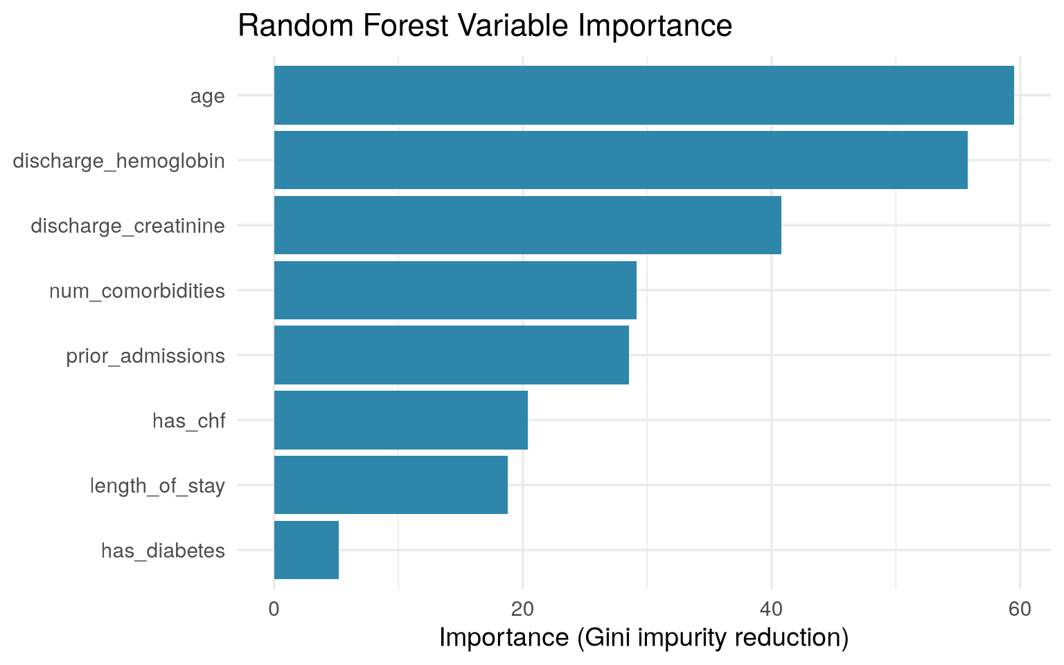
Code
from sklearn.ensemble import RandomForestClassifier
from sklearn.model_selection import cross_val_score, StratifiedKFold
import numpy as np
import pandas as pd
import matplotlib.pyplot as plt

np.random.seed(42)

rf = RandomForestClassifier(
    n_estimators=500,
    max_features='sqrt',
    min_samples_leaf=10,
    oob_score=True,
    random_state=42,
    n_jobs=-1
)
rf.fit(df, y)
RandomForestClassifier(min_samples_leaf=10, n_estimators=500, n_jobs=-1,
oob_score=True, random_state=42)In a Jupyter environment, please rerun this cell to show the HTML representation or trust the notebook. On GitHub, the HTML representation is unable to render, please try loading this page with nbviewer.org.
Parameters
Fitted attributes
Code
importances = pd.Series(rf.feature_importances_, index=feature_names)
importances = importances.sort_values(ascending=True)

fig, ax = plt.subplots(figsize=(8, 5))
importances.plot(kind='barh', ax=ax, color='#2E86AB')
ax.set_xlabel("Importance (Gini impurity reduction)")
ax.set_title("Random Forest Variable Importance")
plt.tight_layout()
plt.show()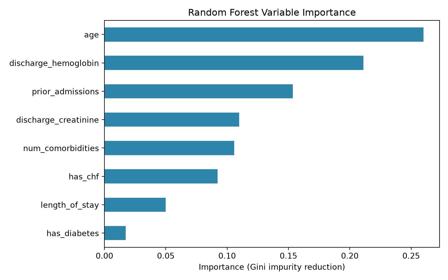
13.4.4 Variable Importance: Two Measures
Impurity-based importance (default): Total reduction in Gini impurity (or variance) from splits on that feature, summed across all trees. Fast but can be biased toward high-cardinality features — that is, variables with many distinct values (a continuous lab value, or an identifier like postcode), as opposed to a low-cardinality variable such as a yes/no flag. Because a high-cardinality feature offers the tree many more candidate split points, it has more chances to look useful by luck, so impurity-based importance can overstate it.
Permutation importance: For each feature, randomly shuffle its values and measure how much the OOB (or test) error increases. More reliable but slower. This is the recommended approach for inference.
WarningVariable Importance Is Not Causal
A feature with high importance in a random forest is predictive of the outcome, not necessarily causally related to it. A correlated proxy (e.g., number of medications as a proxy for disease severity) may appear important even though intervening on it would have no effect. Do not confuse prediction with causation.
13.5 Gradient Boosting
While bagging reduces variance by averaging independent trees, gradient boosting reduces bias by building trees sequentially, where each new tree corrects the mistakes of the previous ensemble.
13.5.1 The Intuition: Learning from Mistakes
- Fit a simple tree to the data.
- Compute the residuals (errors) from this tree.
- Fit a new tree to predict these residuals.
- Add this new tree to the ensemble (scaled by a learning rate).
- Repeat steps 2–4 for \(B\) iterations.
Each new tree focuses on the observations the current ensemble gets wrong. Over many iterations, the ensemble becomes increasingly accurate.
13.5.2 The Mathematics (Brief)
Gradient boosting minimises a loss function \(L(y, \hat{y})\) by gradient descent in function space. At iteration \(m\):
\[\hat{f}_m(x) = \hat{f}_{m-1}(x) + \eta \cdot h_m(x)\]
where \(h_m(x)\) is a tree fitted to the negative gradient of the loss (the “pseudo-residuals”) and \(\eta\) is the learning rate (also called the shrinkage parameter).
13.5.3 XGBoost and LightGBM
In practice, you rarely implement gradient boosting from scratch. Two optimised libraries dominate the landscape:
XGBoost (eXtreme Gradient Boosting) by Chen and Guestrin (2016) added regularisation, efficient computation, and handling of missing values to gradient boosting, making it the dominant algorithm for tabular data competitions and many clinical prediction tasks.
LightGBM by Microsoft further improves efficiency with gradient-based one-side sampling (GOSS) and exclusive feature bundling. It is often faster than XGBoost on large datasets.
Code
library(xgboost)

# Prepare data for xgboost (requires numeric matrix)
X_train <- readmit_data %>%
  select(
    age,
    length_of_stay,
    num_comorbidities,
    prior_admissions,
    discharge_hemoglobin,
    discharge_creatinine,
    has_diabetes,
    has_chf
  ) %>%
  as.matrix()

y_train <- as.numeric(readmit_data$readmitted == "Yes")

dtrain <- xgb.DMatrix(data = X_train, label = y_train)

# Fit XGBoost with cross-validation to find optimal nrounds
set.seed(42)
xgb_cv <- xgb.cv(
  params = list(
    objective = "binary:logistic",
    eval_metric = "auc",
    eta = 0.05,
    max_depth = 4,
    subsample = 0.8,
    colsample_bytree = 0.8
  ),
  data = dtrain,
  nrounds = 1000,
  nfold = 5,
  early_stopping_rounds = 50,
  verbose = 0
)

# xgboost >= 2.0 no longer exposes `$best_iteration` on the CV object, so
# read the best round directly from the evaluation log.
best_nrounds <- which.max(xgb_cv$evaluation_log$test_auc_mean)
cat("Best iteration:", best_nrounds, "\n")
cat("Best CV AUC:", round(max(xgb_cv$evaluation_log$test_auc_mean), 3), "\n")
Code
# Fit final model with optimal nrounds
xgb_model <- xgb.train(
  params = list(
    objective = "binary:logistic",
    eval_metric = "auc",
    eta = 0.05,
    max_depth = 4,
    subsample = 0.8,
    colsample_bytree = 0.8
  ),
  data = dtrain,
  nrounds = best_nrounds,
  verbose = 0
)

# Variable importance
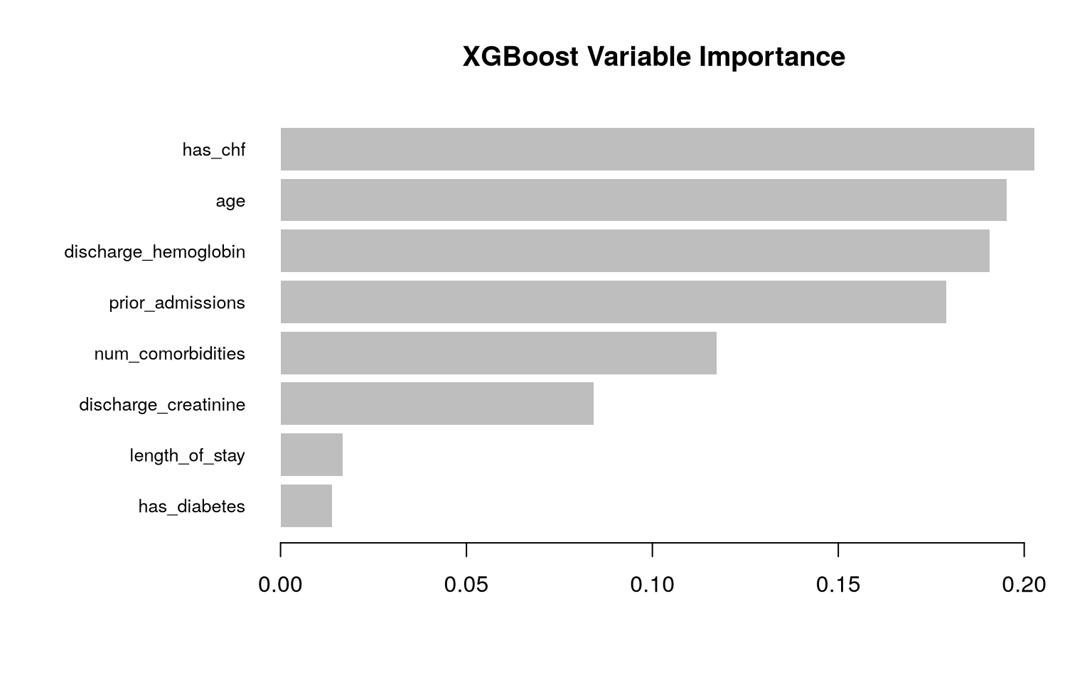
importance_matrix <- xgb.importance(model = xgb_model)
xgb.plot.importance(
  importance_matrix,
  top_n = 8,
  main = "XGBoost Variable Importance"
)
Code
# NOTE: not executed in the book build. Python xgboost (>= 3.x) and R's xgboost
# cannot be loaded in the same knitr/reticulate session without crashing the
# process, so the Python xgboost chunks are shown for reference only. The
# executed R tab above reports the equivalent cross-validated AUC and the
# gain-based variable-importance plot.
import xgboost as xgb
from sklearn.model_selection import cross_val_score, StratifiedKFold
import numpy as np

np.random.seed(42)

# Cross-validation
cv = StratifiedKFold(n_splits=5, shuffle=True, random_state=42)
scores = cross_val_score(
    xgb.XGBClassifier(
        n_estimators=500, learning_rate=0.05, max_depth=4,
        subsample=0.8, colsample_bytree=0.8,
        random_state=42, eval_metric='logloss'
    ),
    df, y, cv=cv, scoring='roc_auc'
)
print(f"XGBoost CV AUC: {scores.mean():.3f} (+/- {scores.std():.3f})")
Code
# Fit and plot importance
xgb_final = xgb.XGBClassifier(
    n_estimators=500, learning_rate=0.05, max_depth=4,
    subsample=0.8, colsample_bytree=0.8,
    random_state=42, eval_metric='logloss'
)
xgb_final.fit(df, y)

fig, ax = plt.subplots(figsize=(8, 5))
xgb.plot_importance(xgb_final, ax=ax, importance_type='gain',
                     title='XGBoost Feature Importance (Gain)')
plt.tight_layout()
plt.show()
13.5.4 Key Hyperparameters
| Parameter | What It Controls | Typical Range |
|---|---|---|
n_estimators / nrounds |
Number of boosting iterations | 100–5000 |
learning_rate / eta |
Step size for each tree | 0.01–0.3 |
max_depth |
Depth of each tree | 3–8 (shallow trees!) |
subsample |
Fraction of data used per tree | 0.5–1.0 |
colsample_bytree |
Fraction of features per tree | 0.5–1.0 |
min_child_weight |
Minimum sum of instance weights in a leaf | 1–10 |
reg_alpha (L1) / reg_lambda (L2) |
Regularisation | 0–10 |
TipThe Learning Rate / Number of Trees Tradeoff
A smaller learning rate requires more trees but generally produces better results. A common strategy: set the learning rate to 0.01–0.05, then tune the number of trees via early stopping (stop when validation error stops improving). XGBoost’s own parameter tuning guide is a practical reference for which knobs to reach for when the model over- or under-fits.
13.6 Hyperparameter Tuning
Let us start from the very beginning, because this idea trips up almost everyone the first time.
When you fit a random forest, there are two completely different kinds of “settings” involved. The first kind, the model learns by itself from the data — for a tree, that means the actual questions at each split (“prior admissions ≥ 2?”). You never choose these; the algorithm finds them. The second kind, you must choose before training even starts — for example, how many trees to grow, or how deep each tree may go. These pre-set dials are called hyperparameters, and the model cannot learn them from the data because they govern how the learning itself happens.
NoteParameters vs. hyperparameters (the one distinction to remember)
- A parameter is something the model estimates from the data (a regression coefficient, a tree’s split rules). You do not set these.
- A hyperparameter is a knob you set beforehand that controls the learning process (number of trees, tree depth, learning rate). The model cannot figure these out on its own.
An analogy: baking bread, the recipe quantities the dough develops into (how the crumb sets) are like parameters — they emerge from the process. The oven temperature and baking time are hyperparameters — you dial them in beforehand, and getting them wrong ruins the loaf no matter how good the dough.
Why bother tuning them? Every library ships with default hyperparameter values, and they are reasonable starting points — but they are generic, not tailored to your dataset. The best settings depend on how much data you have, how noisy it is, and how many predictors there are. Tuning simply means trying several combinations of settings and keeping the one that performs best on held-out data (via the cross-validation you met earlier). Done well, tuning often buys a meaningful bump in performance for free; done carelessly (tuning on the test set), it produces a model that looks great and then disappoints.
The hyperparameters you will see in the code below, in plain language:
| Hyperparameter (R / Python) | What it controls | Rule of thumb |
|---|---|---|
trees / n_estimators |
How many trees are in the forest | More is safer (just slower); a few hundred is usually plenty |
mtry / max_features |
How many predictors each split is allowed to consider | Smaller values make trees more different from each other, which can help |
min_n / min_samples_leaf |
The smallest group of patients allowed in a leaf | Larger values = simpler, smoother trees that overfit less |
max_depth |
How many questions deep a tree may grow | Shallower = simpler; limits overfitting |
You do not need to memorise these — the point is that each one trades flexibility against the risk of overfitting, and tuning finds the sweet spot for your data.
There are two common strategies for searching through the possible combinations.
13.6.1 Grid Search
Grid search means you write down a list of candidate values for each hyperparameter, and the computer tries every possible combination. If you list 4 values for mtry and 5 values for min_n, grid search trains and evaluates all \(4 \times 5 = 20\) combinations and reports which did best. It is thorough and easy to reason about, but the cost explodes as you add hyperparameters: 4 settings each for just five hyperparameters is already \(4^5 = 1024\) models to fit — and each one is itself fit five times under 5-fold cross-validation. This multiplicative blow-up is grid search’s main drawback.
13.6.2 Random Search
Random search instead samples a fixed number of combinations at random from the ranges you specify (say, 20 combinations, regardless of how many hyperparameters there are). Bergstra and Bengio (2012) showed this is usually more efficient than grid search, and the reason is intuitive: in most problems only one or two hyperparameters really matter, but you do not know in advance which. A grid wastes much of its budget trying many values of the unimportant dials while testing only a few values of the important one. Random search, for the same number of model fits, ends up trying more distinct values of every dial — so it is more likely to stumble onto a good value of whichever one actually matters. In practice, start with random search; it gives you most of the benefit for a fraction of the compute.
Code
library(tidymodels)

# Define the model with tunable parameters
rf_spec <- rand_forest(
  trees = 500,
  mtry = tune(),
  min_n = tune()
) %>%
  set_engine("ranger") %>%
  set_mode("classification")

# Create recipe
rf_recipe <- recipe(readmitted ~ ., data = readmit_data)

# Workflow
rf_wf <- workflow() %>%
  add_model(rf_spec) %>%
  add_recipe(rf_recipe)

# Define tuning grid
rf_grid <- grid_random(
  mtry(range = c(2, 7)),
  min_n(range = c(5, 30)),
  size = 20
)

# Cross-validation
set.seed(42)
folds <- vfold_cv(readmit_data, v = 5, strata = readmitted)

# Tune (this may take a moment)
rf_tune_results <- tune_grid(
  rf_wf,
  resamples = folds,
  grid = rf_grid,
  metrics = metric_set(roc_auc)
)

# Best parameters
show_best(rf_tune_results, metric = "roc_auc", n = 5) |>
  knitr::kable(
    digits = 3,
    caption = "Top five random-forest hyperparameter combinations, ranked by cross-validated AUC."
)| mtry | min_n | .metric | .estimator | mean | n | std_err | .config |
|---|---|---|---|---|---|---|---|
| 2 | 29 | roc_auc | binary | 0.777 | 5 | 0.016 | pre0_mod05_post0 |
| 2 | 24 | roc_auc | binary | 0.774 | 5 | 0.016 | pre0_mod04_post0 |
| 2 | 30 | roc_auc | binary | 0.773 | 5 | 0.015 | pre0_mod06_post0 |
| 2 | 14 | roc_auc | binary | 0.771 | 5 | 0.014 | pre0_mod03_post0 |
| 3 | 27 | roc_auc | binary | 0.771 | 5 | 0.016 | pre0_mod09_post0 |
Code
from sklearn.ensemble import RandomForestClassifier
from sklearn.model_selection import RandomizedSearchCV, StratifiedKFold
import numpy as np

np.random.seed(42)

# Define parameter distributions
param_dist = {
    'n_estimators': [100, 200, 500],
    'max_features': ['sqrt', 'log2', 3, 5],
    'min_samples_leaf': [5, 10, 15, 20, 30],
    'max_depth': [5, 10, 15, 20, None]
}

rf = RandomForestClassifier(random_state=42, n_jobs=-1)
cv = StratifiedKFold(n_splits=5, shuffle=True, random_state=42)

# Random search
search = RandomizedSearchCV(
    rf, param_dist, n_iter=20, cv=cv, scoring='roc_auc',
    random_state=42, n_jobs=-1, verbose=0
)
search.fit(df, y)
RandomizedSearchCV(cv=StratifiedKFold(n_splits=5, random_state=42, shuffle=True),
estimator=RandomForestClassifier(n_jobs=-1, random_state=42),
n_iter=20, n_jobs=-1,
param_distributions={'max_depth': [5, 10, 15, 20, None],
'max_features': ['sqrt', 'log2', 3, 5],
'min_samples_leaf': [5, 10, 15, 20, 30],
'n_estimators': [100, 200, 500]},
random_state=42, scoring='roc_auc')In a Jupyter environment, please rerun this cell to show the HTML representation or trust the notebook. On GitHub, the HTML representation is unable to render, please try loading this page with nbviewer.org.
Parameters
Fitted attributes
RandomForestClassifier(max_depth=5, min_samples_leaf=10, n_estimators=500,
n_jobs=-1, random_state=42)Parameters
Fitted attributes
What the code is doing, step by step. Both versions automate the “try many settings, keep the best” recipe. Reading the R version line by line:
rand_forest(... mtry = tune(), min_n = tune())— we declare a random forest but, instead of fixingmtryandmin_n, we mark them withtune(), which is a placeholder meaning “leave this blank for now; we will search for a good value.”- The
recipeandworkflowjust bundle the model with the outcome and predictors — think of the workflow as a sealed envelope containing everything needed to fit the model. grid_random(...)builds the list of 20 random combinations ofmtryandmin_nto try (these are the candidate “oven settings”).vfold_cv(...)creates the 5-fold cross-validation splits. This is the crucial part: every candidate setting is judged on held-out patients, not on the data it was trained on. That is what stops us from simply picking the most complex, overfit model.tune_grid(...)does the heavy lifting — it fits the forest for each of the 20 settings, across all 5 folds, and records the cross-validated AUC for each.show_best(...)then prints the top settings.
What the output shows. show_best returns a small table: each row is one hyperparameter combination, with its mean cross-validated AUC and the spread across folds. You read it top-down — the first row is the winning combination. select_best grabs that winner, and finalize_workflow + fit retrain the forest on all the data using those best settings, giving you the final model. The Python RandomizedSearchCV does exactly the same thing in one object, printing Best AUC and the Best parameters dictionary at the end. The specific numbers are not the lesson (the data here are simulated); the lesson is the workflow: define the dials to search, score each candidate honestly on held-out folds, and keep the winner.
ImportantThe cardinal rule of tuning
Tuning must happen inside cross-validation, using only the training data — never tune by looking at your final test set. If you try hundreds of settings and pick the one that scores best on the test set, that test score is no longer an honest estimate of future performance: you have, in effect, let the test set leak into model development. Keep a truly untouched test set (or external validation data) for the final check, after all tuning is done.
13.7 Comparing Methods: When to Use What
| Method | Strengths | Weaknesses | Best For |
|---|---|---|---|
| Single tree | Interpretable, handles non-linearity | Unstable, overfits | Exploration, simple rules |
| Random forest | Robust, low tuning needed, OOB error | Less interpretable than single tree | General-purpose prediction |
| Gradient boosting | Often highest accuracy, flexible | More tuning, can overfit, slower | Maximising prediction accuracy |
| Logistic regression | Interpretable, well-understood inference | Assumes linearity (without transforms) | Inference, small samples, reporting ORs |
NotePractical Advice for Clinical Prediction Models
Start with logistic regression as your baseline. If you need better prediction and have enough data (typically hundreds of events), try a random forest. If you want to squeeze out the last bit of performance and are willing to tune carefully, use XGBoost. Always compare against the logistic regression baseline — if the improvement is marginal, prefer the simpler model.
13.8 Clinical Example: Readmission Risk Stratification
Let us bring everything together by comparing all three methods on the hospital readmission dataset.
Note how the data are handled: rather than carving off a single train/test split, we pass the whole dataset to 10-fold cross-validation (vfold_cv in R, StratifiedKFold in Python), and every model is scored the same way — trained on 9 folds and evaluated on the held-out fold, rotated ten times. This keeps the comparison fair (all three models see identical folds) and uses the data efficiently. A separate untouched test set (or external data) would still be needed for a final performance estimate once a model is chosen, as stressed in the tuning section above.
Code
library(tidyverse)   # ggplot2 / dplyr / tibble
library(tidymodels)

set.seed(42)
folds <- vfold_cv(readmit_data, v = 10, strata = readmitted)

# Logistic regression
lr_spec <- logistic_reg() %>% set_engine("glm")
lr_wf <- workflow() %>%
  add_model(lr_spec) %>%
  add_recipe(recipe(readmitted ~ ., data = readmit_data))
lr_res <- fit_resamples(lr_wf, resamples = folds, metrics = metric_set(roc_auc))

# Random forest
rf_spec <- rand_forest(trees = 500, mtry = 3, min_n = 10) %>%
  set_engine("ranger") %>%
  set_mode("classification")
rf_wf <- workflow() %>%
  add_model(rf_spec) %>%
  add_recipe(recipe(readmitted ~ ., data = readmit_data))
rf_res <- fit_resamples(rf_wf, resamples = folds, metrics = metric_set(roc_auc))

# Boosted trees (via xgboost engine in tidymodels)
xgb_spec <- boost_tree(
  trees = 500,
  tree_depth = 4,
  learn_rate = 0.05,
  min_n = 10
) %>%
  set_engine("xgboost") %>%
  set_mode("classification")
xgb_wf <- workflow() %>%
  add_model(xgb_spec) %>%
  add_recipe(recipe(readmitted ~ ., data = readmit_data))
xgb_res <- fit_resamples(
  xgb_wf,
  resamples = folds,
  metrics = metric_set(roc_auc)
)

# Collect and compare results
bind_rows(
  collect_metrics(lr_res) %>% mutate(model = "Logistic Regression"),
  collect_metrics(rf_res) %>% mutate(model = "Random Forest"),
  collect_metrics(xgb_res) %>% mutate(model = "XGBoost")
) %>%
  select(model, .metric, mean, std_err) %>%
  arrange(desc(mean)) %>%
  knitr::kable(
    digits = 3,
    caption = "Cross-validated AUC (mean +/- standard error) for the three models."
)| model | .metric | mean | std_err |
|---|---|---|---|
| Logistic Regression | roc_auc | 0.790 | 0.013 |
| Random Forest | roc_auc | 0.765 | 0.012 |
| XGBoost | roc_auc | 0.730 | 0.016 |
Code
from sklearn.linear_model import LogisticRegression
from sklearn.ensemble import RandomForestClassifier, GradientBoostingClassifier
from sklearn.model_selection import cross_val_score, StratifiedKFold
from sklearn.preprocessing import StandardScaler
from sklearn.pipeline import make_pipeline
import numpy as np
import pandas as pd

np.random.seed(42)
cv = StratifiedKFold(n_splits=10, shuffle=True, random_state=42)

models = {
    "Logistic Regression": make_pipeline(
        StandardScaler(), LogisticRegression(max_iter=1000)
    ),
    "Random Forest": RandomForestClassifier(
        n_estimators=500, min_samples_leaf=10, random_state=42, n_jobs=-1
    ),
    "Gradient Boosting": GradientBoostingClassifier(
        n_estimators=500,
        learning_rate=0.05,
        max_depth=4,
        subsample=0.8,
        random_state=42,
    ),
}

results = []
for name, model in models.items():
    scores = cross_val_score(model, df, y, cv=cv, scoring="roc_auc")
    results.append(
        {
            "Model": name,
            "Mean AUC": f"{scores.mean():.3f}",
            "Std": f"{scores.std():.3f}",
        }
    )
    print(f"{name:25s}: AUC = {scores.mean():.3f} (+/- {scores.std():.3f})")

print(pd.DataFrame(results).to_string(index=False))
Logistic Regression : AUC = 0.807 (+/- 0.051)
Random Forest : AUC = 0.782 (+/- 0.061)
Gradient Boosting : AUC = 0.738 (+/- 0.071)
Model Mean AUC Std
Logistic Regression 0.807 0.051
Random Forest 0.782 0.061
Gradient Boosting 0.738 0.071What the code is doing, and what the output shows. Both versions fit the same three models — logistic regression, a random forest, and gradient boosting (XGBoost in R, scikit-learn’s gradient boosting in Python) — under one identical 10-fold cross-validation, then collect each model’s cross-validated AUC. The code prints a small table with one row per model: its mean AUC across the ten folds and the spread (std_err / Std) around that mean, sorted best-first. Read it as a leaderboard, but a cautious one: compare the gap between models against the spread. If the top two models are within a standard error or so of each other, they are effectively tied, and the practical choice should then favour the simpler, more interpretable model — which is exactly the advice in the callout above. On these simulated data the three tend to land close together, reinforcing the point that a fancier model is not automatically a better one.
13.9 Exercises
TipExercise 1: Build and Prune a Classification Tree
Using the readmission dataset (or a dataset of your choice):
- Fit a full, unpruned classification tree. How many terminal nodes does it have?
- Use cross-validation to find the optimal complexity parameter (cp in R) or maximum depth (in Python).
- Prune the tree and plot it. How does it compare to the full tree?
- What are the top 3 splitting variables? Do they make clinical sense?
Code
library(rpart) # rpart(), rpart.control()
library(rpart.plot) # rpart.plot() for visualising the tree

# Fit a full tree (set cp very low to avoid early pruning)
full_tree <- rpart(
  readmitted ~ .,
  data = readmit_data,
  method = "class",
  control = rpart.control(cp = 0.001)
)

# Your code:
# 1. Count terminal nodes
# 2. Use printcp() and plotcp() to find optimal cp
# 3. Prune and plot
# 4. Examine variable importance: full_tree$variable.importance
NoteSolution
Code
# =============================================================================
# Chapter 8, Exercise 1: Build and Prune a Classification Tree
# 1. Fit a full, unpruned tree and count terminal nodes.
# 2. Use cross-validation to find the optimal cp.
# 3. Prune the tree and plot it.
# 4. Identify the top 3 splitting variables.
# =============================================================================

library(tidyverse)
library(rpart)
library(rpart.plot)

# --- Simulate the readmission dataset (same as chapter) ---
set.seed(42)
n <- 1000

readmit_data <- tibble(
  age = rnorm(n, 68, 12),
  length_of_stay = rpois(n, 5) + 1,
  num_comorbidities = rpois(n, 3),
  prior_admissions = rpois(n, 1),
  discharge_hemoglobin = rnorm(n, 11, 2),
  discharge_creatinine = rlnorm(n, 0.2, 0.5),
  has_diabetes = rbinom(n, 1, 0.35),
  has_chf = rbinom(n, 1, 0.25),
  readmitted = factor(
    rbinom(n, 1, plogis(-3 + 0.02 * (rnorm(n, 68, 12) - 68) +
                          0.15 * rpois(n, 1) +
                          0.1 * rpois(n, 3) +
                          0.3 * rbinom(n, 1, 0.25) -
                          0.1 * rnorm(n, 11, 2))),
    labels = c("No", "Yes")
  )
)

cat("Readmission rate:", mean(readmit_data$readmitted == "Yes"), "\n")

# --- Part 1: Fit a full, unpruned tree ---
full_tree <- rpart(readmitted ~ ., data = readmit_data, method = "class",
                   control = rpart.control(cp = 0.001, minsplit = 2, minbucket = 1))

n_terminal_full <- sum(full_tree$frame$var == "<leaf>")
cat("\nFull tree terminal nodes:", n_terminal_full, "\n")

# --- Part 2: Cross-validation to find optimal cp ---
cat("\nCP Table:\n")
printcp(full_tree)

# Plot CV error vs cp
plotcp(full_tree)

# Find optimal cp (minimum xerror)
cp_table <- full_tree$cptable
optimal_cp <- cp_table[which.min(cp_table[, "xerror"]), "CP"]
cat("\nOptimal cp:", optimal_cp, "\n")

# Alternative: 1-SE rule (smallest tree within 1 SE of the minimum)
min_xerror <- min(cp_table[, "xerror"])
min_se <- cp_table[which.min(cp_table[, "xerror"]), "xstd"]
cp_1se <- cp_table[cp_table[, "xerror"] <= min_xerror + min_se, "CP"]
optimal_cp_1se <- max(cp_1se)  # largest cp (smallest tree) within 1 SE
cat("Optimal cp (1-SE rule):", optimal_cp_1se, "\n")

# --- Part 3: Prune and plot ---
pruned_tree <- prune(full_tree, cp = optimal_cp)
n_terminal_pruned <- sum(pruned_tree$frame$var == "<leaf>")
cat("\nPruned tree terminal nodes:", n_terminal_pruned, "\n")

rpart.plot(pruned_tree, type = 4, extra = 106, under = TRUE,
           box.palette = "RdYlGn", roundint = FALSE,
           main = "Pruned Decision Tree: 30-Day Readmission")

# --- Part 4: Top 3 splitting variables ---
cat("\nVariable Importance:\n")
vi <- sort(full_tree$variable.importance, decreasing = TRUE)
print(vi)

top3 <- names(vi)[1:min(3, length(vi))]
cat("\nTop 3 splitting variables:", paste(top3, collapse = ", "), "\n")
cat("\nClinical interpretation:\n")
cat("- These variables capture patient acuity and complexity.\n")
cat("- Discharge lab values (hemoglobin, creatinine) reflect the patient's\n")
cat("  clinical status at the time of discharge.\n")
cat("- Age, comorbidity count, and prior admissions reflect overall\n")
cat("  disease burden and frailty.\n")
cat("- These are well-established risk factors for 30-day readmission\n")
cat("  in the clinical literature.\n")
Code
# =============================================================================
# Chapter 8, Exercise 1: Build and Prune a Classification Tree
# 1. Fit trees with different max_depth values and count leaves.
# 2. Cross-validate each to find optimal max_depth.
# 3. Plot the optimal tree.
# 4. Examine feature importances.
# =============================================================================

import numpy as np
import pandas as pd
from sklearn.tree import DecisionTreeClassifier, plot_tree
from sklearn.model_selection import cross_val_score, StratifiedKFold
import matplotlib.pyplot as plt

# --- Simulate the readmission dataset (same as chapter) ---
np.random.seed(42)
n = 1000

df = pd.DataFrame({
    'age': np.random.normal(68, 12, n),
    'length_of_stay': np.random.poisson(5, n) + 1,
    'num_comorbidities': np.random.poisson(3, n),
    'prior_admissions': np.random.poisson(1, n),
    'discharge_hemoglobin': np.random.normal(11, 2, n),
    'discharge_creatinine': np.random.lognormal(0.2, 0.5, n),
    'has_diabetes': np.random.binomial(1, 0.35, n),
    'has_chf': np.random.binomial(1, 0.25, n)
})
y = np.random.binomial(1, 0.18, n)

feature_names = list(df.columns)
print(f"Readmission rate: {y.mean():.3f}")

# --- Part 1: Fit a full, unpruned tree ---
full_tree = DecisionTreeClassifier(random_state=42)
full_tree.fit(df, y)
n_leaves_full = full_tree.get_n_leaves()
print(f"\nFull (unpruned) tree: {n_leaves_full} terminal nodes")
print(f"Full tree depth: {full_tree.get_depth()}")

# --- Part 2: Cross-validation to find optimal max_depth ---
depths = [2, 3, 4, 5, 7, 10, 15, 20, None]
cv = StratifiedKFold(n_splits=10, shuffle=True, random_state=42)

print("\nCross-validation results by max_depth:")
print(f"{'max_depth':>10s}  {'Mean AUC':>10s}  {'Std AUC':>10s}")
print("-" * 35)

cv_results = []
for d in depths:
    tree = DecisionTreeClassifier(max_depth=d, random_state=42)
    scores = cross_val_score(tree, df, y, cv=cv, scoring='roc_auc')
    label = str(d) if d is not None else "None"
    cv_results.append({'max_depth': d, 'label': label,
                       'mean_auc': scores.mean(), 'std_auc': scores.std()})
    print(f"{label:>10s}  {scores.mean():>10.3f}  {scores.std():>10.3f}")

# Find the best depth
best = max(cv_results, key=lambda x: x['mean_auc'])
print(f"\nBest max_depth: {best['label']} (AUC = {best['mean_auc']:.3f})")

# --- Part 3: Fit and plot the optimal tree ---
best_depth = best['max_depth']
optimal_tree = DecisionTreeClassifier(max_depth=best_depth, random_state=42)
optimal_tree.fit(df, y)

print(f"\nOptimal tree: {optimal_tree.get_n_leaves()} terminal nodes")

fig, ax = plt.subplots(figsize=(20, 10))
plot_tree(optimal_tree, feature_names=feature_names, class_names=['No', 'Yes'],
          filled=True, rounded=True, ax=ax, fontsize=9,
          max_depth=4)  # show up to depth 4 for readability
ax.set_title(f"Pruned Decision Tree (max_depth={best['label']})")
plt.tight_layout()
plt.show()

# --- Part 4: Top 3 splitting variables ---
importances = pd.Series(optimal_tree.feature_importances_, index=feature_names)
importances = importances.sort_values(ascending=False)

print("\nFeature Importances:")
print(importances.to_string())

top3 = importances.head(3).index.tolist()
print(f"\nTop 3 splitting variables: {top3}")

# Plot feature importances
fig, ax = plt.subplots(figsize=(8, 5))
importances.sort_values(ascending=True).plot(kind='barh', ax=ax, color='#2E86AB')
ax.set_xlabel("Feature Importance (Gini)")
ax.set_title("Decision Tree Feature Importance")
plt.tight_layout()
plt.show()

print("\nClinical interpretation:")
print("- These variables capture patient acuity and complexity.")
print("- Discharge lab values reflect the patient's clinical status at discharge.")
print("- Age, comorbidity count, and prior admissions reflect disease burden.")
print("- These are well-established readmission risk factors in the literature.")
TipExercise 2: Random Forest vs XGBoost Tuning Challenge
- Split the readmission data into 80% training and 20% test sets.
- Using the training set with 5-fold cross-validation:
- Tune a random forest (try different
mtry/max_featuresandmin_n/min_samples_leafvalues). - Tune an XGBoost model (try different
learning_rate,max_depth, andn_estimatorsvalues).
- Tune a random forest (try different
- Select the best hyperparameters for each model.
- Evaluate both models on the held-out test set. Which performs better?
- Create variable importance plots for both models. Do they agree on the most important features?
Code
library(tidymodels) # initial_split(), training(), testing(), tune_grid()

# Split data
set.seed(42)
split <- initial_split(readmit_data, prop = 0.8, strata = readmitted)
train <- training(split)
test <- testing(split)

# Your code: define models with tune(), create grids, run tune_grid()
# Finalize models, predict on test set, compare
Code
from sklearn.model_selection import train_test_split, RandomizedSearchCV
from sklearn.ensemble import RandomForestClassifier
import xgboost as xgb

X_train, X_test, y_train, y_test = train_test_split(
    df, y, test_size=0.2, stratify=y, random_state=42
)

# Your code: define param_dist for RF and XGBoost
# Run RandomizedSearchCV for each
# Evaluate on test set with roc_auc_score
NoteSolution
Code
# =============================================================================
# Chapter 8, Exercise 2: Random Forest vs XGBoost Tuning Challenge
# 1. Split data 80/20. 2. Tune RF and XGBoost with 5-fold CV.
# 3. Select best hyperparameters. 4. Evaluate on test set.
# 5. Create variable importance plots.
# =============================================================================

library(tidyverse)
library(tidymodels)

# --- Simulate the readmission dataset (same as chapter) ---
set.seed(42)
n <- 1000

readmit_data <- tibble(
  age = rnorm(n, 68, 12),
  length_of_stay = rpois(n, 5) + 1,
  num_comorbidities = rpois(n, 3),
  prior_admissions = rpois(n, 1),
  discharge_hemoglobin = rnorm(n, 11, 2),
  discharge_creatinine = rlnorm(n, 0.2, 0.5),
  has_diabetes = rbinom(n, 1, 0.35),
  has_chf = rbinom(n, 1, 0.25),
  readmitted = factor(
    rbinom(n, 1, plogis(-3 + 0.02 * (rnorm(n, 68, 12) - 68) +
                          0.15 * rpois(n, 1) +
                          0.1 * rpois(n, 3) +
                          0.3 * rbinom(n, 1, 0.25) -
                          0.1 * rnorm(n, 11, 2))),
    labels = c("No", "Yes")
  )
)

# --- Part 1: Train/test split ---
set.seed(42)
split <- initial_split(readmit_data, prop = 0.8, strata = readmitted)
train <- training(split)
test  <- testing(split)

cat("Training set size:", nrow(train), "\n")
cat("Test set size:", nrow(test), "\n")

# 5-fold CV on training set
folds <- vfold_cv(train, v = 5, strata = readmitted)

# Recipe (shared)
base_recipe <- recipe(readmitted ~ ., data = train)

# --- Part 2a: Tune Random Forest ---
rf_spec <- rand_forest(
  trees = 500,
  mtry = tune(),
  min_n = tune()
) %>%
  set_engine("ranger", importance = "impurity") %>%
  set_mode("classification")

rf_wf <- workflow() %>%
  add_model(rf_spec) %>%
  add_recipe(base_recipe)

rf_grid <- grid_regular(
  mtry(range = c(2, 7)),
  min_n(range = c(5, 30)),
  levels = 5
)

set.seed(42)
rf_tune <- tune_grid(rf_wf, resamples = folds, grid = rf_grid,
                     metrics = metric_set(roc_auc))

cat("\n--- Random Forest Tuning Results (Top 5) ---\n")
print(show_best(rf_tune, metric = "roc_auc", n = 5))

best_rf <- select_best(rf_tune, metric = "roc_auc")
cat("\nBest RF params - mtry:", best_rf$mtry, "min_n:", best_rf$min_n, "\n")

# --- Part 2b: Tune XGBoost ---
xgb_spec <- boost_tree(
  trees = 500,
  tree_depth = tune(),
  learn_rate = tune(),
  min_n = tune()
) %>%
  set_engine("xgboost") %>%
  set_mode("classification")

xgb_wf <- workflow() %>%
  add_model(xgb_spec) %>%
  add_recipe(base_recipe)

xgb_grid <- grid_regular(
  tree_depth(range = c(2, 6)),
  learn_rate(range = c(-3, -1)),   # log10 scale: 0.001 to 0.1
  min_n(range = c(5, 20)),
  levels = 4
)

set.seed(42)
xgb_tune <- tune_grid(xgb_wf, resamples = folds, grid = xgb_grid,
                      metrics = metric_set(roc_auc))

cat("\n--- XGBoost Tuning Results (Top 5) ---\n")
print(show_best(xgb_tune, metric = "roc_auc", n = 5))

best_xgb <- select_best(xgb_tune, metric = "roc_auc")
cat("\nBest XGB params - depth:", best_xgb$tree_depth,
    "learn_rate:", best_xgb$learn_rate,
    "min_n:", best_xgb$min_n, "\n")

# --- Part 3: Finalize and fit on full training set ---
final_rf_wf <- finalize_workflow(rf_wf, best_rf)
final_xgb_wf <- finalize_workflow(xgb_wf, best_xgb)

rf_final_fit <- fit(final_rf_wf, data = train)
xgb_final_fit <- fit(final_xgb_wf, data = train)

# --- Part 4: Evaluate on test set ---
rf_test_pred  <- predict(rf_final_fit, test, type = "prob") %>%
  bind_cols(test %>% select(readmitted))
xgb_test_pred <- predict(xgb_final_fit, test, type = "prob") %>%
  bind_cols(test %>% select(readmitted))

rf_auc  <- roc_auc(rf_test_pred, truth = readmitted, .pred_Yes)
xgb_auc <- roc_auc(xgb_test_pred, truth = readmitted, .pred_Yes)

cat("\n=== Test Set Performance ===\n")
cat("Random Forest AUC:", rf_auc$.estimate, "\n")
cat("XGBoost AUC:      ", xgb_auc$.estimate, "\n")

if (xgb_auc$.estimate > rf_auc$.estimate) {
  cat("\nXGBoost performs better on the test set.\n")
} else {
  cat("\nRandom Forest performs better on the test set.\n")
}

# --- Part 5: Variable importance plots ---
# NOTE: the `vip` package was archived from CRAN and is no longer installable,
# so we read the importance scores straight out of the fitted engine objects
# and plot them ourselves. This is a few more lines but has no dependency and
# makes it obvious which importance measure is being shown.

importance_plot <- function(scores, title) {
  tibble(variable = names(scores), importance = as.numeric(scores)) |>
    slice_max(importance, n = 8) |>
    ggplot(aes(x = importance, y = reorder(variable, importance))) +
    geom_col(fill = "steelblue") +
    labs(x = "Importance", y = NULL, title = title) +
    theme_minimal()
}

# Random Forest: ranger stores impurity importance because the spec above set
# `importance = "impurity"`.
rf_scores <- rf_final_fit |>
  extract_fit_engine() |>
  (\(x) x$variable.importance)()
print(importance_plot(rf_scores, "Random Forest variable importance (impurity)"))

# XGBoost: xgb.importance() returns a data frame, so reshape it to a named vector.
xgb_imp <- xgboost::xgb.importance(model = extract_fit_engine(xgb_final_fit))
xgb_scores <- setNames(xgb_imp$Gain, xgb_imp$Feature)
print(importance_plot(xgb_scores, "XGBoost variable importance (gain)"))

cat("\nBoth models should generally agree on the most important features,\n")
cat("though rankings may differ. Continuous variables with more possible\n")
cat("split points (e.g., age, creatinine) often rank higher in tree-based\n")
cat("importance measures than binary variables (e.g., has_chf).\n")
Code
# =============================================================================
# Chapter 8, Exercise 2: Random Forest vs XGBoost Tuning Challenge
# 1. Split data 80/20. 2. Tune RF and XGBoost with 5-fold CV.
# 3. Select best hyperparameters. 4. Evaluate on test set.
# 5. Create variable importance plots.
# =============================================================================

import numpy as np
import pandas as pd
from sklearn.model_selection import (train_test_split, RandomizedSearchCV,
                                      StratifiedKFold)
from sklearn.ensemble import RandomForestClassifier
from sklearn.metrics import roc_auc_score
import xgboost as xgb
import matplotlib.pyplot as plt

# --- Simulate the readmission dataset (same as chapter) ---
np.random.seed(42)
n = 1000

df = pd.DataFrame({
    'age': np.random.normal(68, 12, n),
    'length_of_stay': np.random.poisson(5, n) + 1,
    'num_comorbidities': np.random.poisson(3, n),
    'prior_admissions': np.random.poisson(1, n),
    'discharge_hemoglobin': np.random.normal(11, 2, n),
    'discharge_creatinine': np.random.lognormal(0.2, 0.5, n),
    'has_diabetes': np.random.binomial(1, 0.35, n),
    'has_chf': np.random.binomial(1, 0.25, n)
})
y = np.random.binomial(1, 0.18, n)

feature_names = list(df.columns)

# --- Part 1: Train/test split ---
X_train, X_test, y_train, y_test = train_test_split(
    df, y, test_size=0.2, stratify=y, random_state=42
)
print(f"Training set: {X_train.shape[0]} | Test set: {X_test.shape[0]}")

cv = StratifiedKFold(n_splits=5, shuffle=True, random_state=42)

# --- Part 2a: Tune Random Forest ---
rf_param_dist = {
    'n_estimators': [200, 500],
    'max_features': ['sqrt', 'log2', 3, 5, 7],
    'min_samples_leaf': [5, 10, 15, 20, 30],
    'max_depth': [5, 10, 15, 20, None]
}

rf = RandomForestClassifier(random_state=42, n_jobs=-1)

rf_search = RandomizedSearchCV(
    rf, rf_param_dist, n_iter=30, cv=cv, scoring='roc_auc',
    random_state=42, n_jobs=-1, verbose=0
)
rf_search.fit(X_train, y_train)

print(f"\n--- Random Forest Tuning ---")
print(f"Best CV AUC: {rf_search.best_score_:.3f}")
print(f"Best params: {rf_search.best_params_}")

# --- Part 2b: Tune XGBoost ---
xgb_param_dist = {
    'n_estimators': [200, 500, 1000],
    'learning_rate': [0.01, 0.05, 0.1],
    'max_depth': [2, 3, 4, 5, 6],
    'subsample': [0.7, 0.8, 0.9, 1.0],
    'colsample_bytree': [0.7, 0.8, 0.9, 1.0],
    'min_child_weight': [1, 5, 10]
}

xgb_model = xgb.XGBClassifier(
    random_state=42, use_label_encoder=False, eval_metric='logloss'
)

xgb_search = RandomizedSearchCV(
    xgb_model, xgb_param_dist, n_iter=30, cv=cv, scoring='roc_auc',
    random_state=42, n_jobs=-1, verbose=0
)
xgb_search.fit(X_train, y_train)

print(f"\n--- XGBoost Tuning ---")
print(f"Best CV AUC: {xgb_search.best_score_:.3f}")
print(f"Best params: {xgb_search.best_params_}")

# --- Part 4: Evaluate on test set ---
rf_best = rf_search.best_estimator_
xgb_best = xgb_search.best_estimator_

rf_test_probs = rf_best.predict_proba(X_test)[:, 1]
xgb_test_probs = xgb_best.predict_proba(X_test)[:, 1]

rf_test_auc = roc_auc_score(y_test, rf_test_probs)
xgb_test_auc = roc_auc_score(y_test, xgb_test_probs)

print(f"\n=== Test Set Performance ===")
print(f"Random Forest AUC: {rf_test_auc:.3f}")
print(f"XGBoost AUC:       {xgb_test_auc:.3f}")

if xgb_test_auc > rf_test_auc:
    print("\nXGBoost performs better on the test set.")
else:
    print("\nRandom Forest performs better on the test set.")

# --- Part 5: Variable importance plots ---
fig, axes = plt.subplots(1, 2, figsize=(14, 5))

# Random Forest importance
rf_imp = pd.Series(rf_best.feature_importances_, index=feature_names)
rf_imp = rf_imp.sort_values(ascending=True)
rf_imp.plot(kind='barh', ax=axes[0], color='#2E86AB')
axes[0].set_xlabel("Feature Importance (Gini)")
axes[0].set_title("Random Forest Variable Importance")

# XGBoost importance
xgb_imp = pd.Series(xgb_best.feature_importances_, index=feature_names)
xgb_imp = xgb_imp.sort_values(ascending=True)
xgb_imp.plot(kind='barh', ax=axes[1], color='#D55E00')
axes[1].set_xlabel("Feature Importance (Gain)")
axes[1].set_title("XGBoost Variable Importance")

plt.tight_layout()
plt.show()

# Compare top features
print("\nRF top 3 features:", rf_imp.sort_values(ascending=False).head(3).index.tolist())
print("XGB top 3 features:", xgb_imp.sort_values(ascending=False).head(3).index.tolist())
print("\nBoth models should generally agree on the most important features,")
print("though rankings may differ due to how each algorithm uses features.")
TipExercise 3: Interpreting a Clinical Prediction Model
You have built a gradient-boosted model for 30-day hospital readmission. Your hospital administration asks you to present the results.
- Write a non-technical summary (3–4 sentences) explaining what the model does and how well it performs, suitable for a hospital quality committee.
- The model identifies “number of prior admissions” and “discharge creatinine” as the two most important predictors. Explain to a clinical audience what this means and does not mean (recall the caution about variable importance and causation).
- How would you propose to validate this model before deploying it in clinical practice? What could go wrong if you skip external validation?
NoteSolution
Code
# =============================================================================
# Chapter 8, Exercise 3: Interpreting a Clinical Prediction Model
# Conceptual exercise: write answers as comments.
# =============================================================================

# =============================================================================
# Part 1: Non-technical summary for a hospital quality committee
# =============================================================================
#
# "We developed a computer-based prediction model that estimates each patient's
# risk of being readmitted to the hospital within 30 days of discharge. The
# model uses information routinely collected during hospitalisation -- such as
# lab values, age, prior admissions, and existing medical conditions -- to
# assign each patient a risk score between 0% and 100%. In cross-validated
# testing, the model correctly distinguished between patients who were and
# were not readmitted approximately [AUC]% of the time. This tool could help
# care teams focus discharge planning resources on the patients at highest
# risk, potentially reducing readmission rates and associated penalties."

# =============================================================================
# Part 2: Explaining variable importance to a clinical audience
# =============================================================================
#
# "The model identified 'number of prior admissions' and 'discharge creatinine'
# as the two variables that contribute most to the model's predictions. This
# means that knowing these values provides the most useful information for
# distinguishing patients who will be readmitted from those who will not.
#
# WHAT THIS MEANS:
# - Patients with more prior admissions tend to have higher predicted risk.
# - Patients with elevated discharge creatinine (indicating impaired kidney
#   function) also tend to have higher predicted risk.
# - These findings align with clinical intuition: patients with a history of
#   recurrent hospitalisations and those with renal impairment are known to
#   be at elevated risk.
#
# WHAT THIS DOES NOT MEAN:
# - Variable importance does NOT imply causation. We cannot say that reducing
#   creatinine at discharge will reduce readmission risk. The model identifies
#   associations, not causes.
# - A variable with high importance may be a proxy for something else. For
#   example, 'prior admissions' may reflect underlying disease severity,
#   social determinants, or healthcare access patterns rather than being
#   a direct cause of readmission.
# - We should not intervene on these variables based on importance alone.
#   Clinical trials or causal inference methods would be needed to establish
#   whether modifying these factors actually changes outcomes."

# =============================================================================
# Part 3: Validation strategy before clinical deployment
# =============================================================================
#
# PROPOSED VALIDATION PLAN:
#
# 1. Temporal validation: Test the model on data from a time period AFTER the
#    training data (e.g., train on 2020-2022, validate on 2023-2024). This
#    tests whether the model's performance holds over time, as clinical
#    practices and patient populations may shift.
#
# 2. External validation: Apply the model to data from a different hospital
#    system. A model developed at one institution may not generalise to
#    another due to differences in patient demographics, coding practices,
#    discharge protocols, and local disease patterns.
#
# 3. Subgroup analysis: Evaluate performance across key demographic groups
#    (age, sex, race/ethnicity, insurance status). A model that performs
#    well overall but poorly for specific populations could worsen existing
#    health disparities.
#
# 4. Calibration assessment: Verify that predicted probabilities match
#    observed readmission rates. A model that says "30% risk" should be
#    right about 30% of the time across all risk levels.
#
# 5. Prospective pilot: Before full deployment, run the model in parallel
#    alongside current practice (silent mode) to monitor performance in
#    real-time without affecting clinical decisions.
#
# RISKS OF SKIPPING EXTERNAL VALIDATION:
# - The model may be overfit to idiosyncrasies of the development data
#   (specific EMR system, local coding conventions, patient mix).
# - Performance reported from internal validation (even cross-validation)
#   tends to be optimistically biased.
# - Deploying an unvalidated model could misallocate resources, either
#   missing high-risk patients (false negatives) or overwhelming care
#   teams with false alarms (false positives).
# - Regulatory and ethical risks: deploying a model without adequate
#   validation may violate institutional policies and could cause patient
#   harm.

cat("This exercise is conceptual. See the comments in this file for the\n")
cat("complete answers to all three parts.\n")
Code
# =============================================================================
# Chapter 8, Exercise 3: Interpreting a Clinical Prediction Model
# Conceptual exercise: write answers as comments.
# =============================================================================

# =============================================================================
# Part 1: Non-technical summary for a hospital quality committee
# =============================================================================
#
# "We developed a computer-based prediction model that estimates each patient's
# risk of being readmitted to the hospital within 30 days of discharge. The
# model uses information routinely collected during hospitalisation -- such as
# lab values, age, prior admissions, and existing medical conditions -- to
# assign each patient a risk score between 0% and 100%. In cross-validated
# testing, the model correctly distinguished between patients who were and
# were not readmitted approximately [AUC]% of the time. This tool could help
# care teams focus discharge planning resources on the patients at highest
# risk, potentially reducing readmission rates and associated penalties."

# =============================================================================
# Part 2: Explaining variable importance to a clinical audience
# =============================================================================
#
# "The model identified 'number of prior admissions' and 'discharge creatinine'
# as the two variables that contribute most to the model's predictions. This
# means that knowing these values provides the most useful information for
# distinguishing patients who will be readmitted from those who will not.
#
# WHAT THIS MEANS:
# - Patients with more prior admissions tend to have higher predicted risk.
# - Patients with elevated discharge creatinine (indicating impaired kidney
#   function) also tend to have higher predicted risk.
# - These findings align with clinical intuition: patients with a history of
#   recurrent hospitalisations and those with renal impairment are known to
#   be at elevated risk.
#
# WHAT THIS DOES NOT MEAN:
# - Variable importance does NOT imply causation. We cannot say that reducing
#   creatinine at discharge will reduce readmission risk. The model identifies
#   associations, not causes.
# - A variable with high importance may be a proxy for something else. For
#   example, 'prior admissions' may reflect underlying disease severity,
#   social determinants, or healthcare access patterns rather than being
#   a direct cause of readmission.
# - We should not intervene on these variables based on importance alone.
#   Clinical trials or causal inference methods would be needed to establish
#   whether modifying these factors actually changes outcomes."

# =============================================================================
# Part 3: Validation strategy before clinical deployment
# =============================================================================
#
# PROPOSED VALIDATION PLAN:
#
# 1. Temporal validation: Test the model on data from a time period AFTER the
#    training data (e.g., train on 2020-2022, validate on 2023-2024). This
#    tests whether the model's performance holds over time.
#
# 2. External validation: Apply the model to data from a different hospital
#    system. A model developed at one institution may not generalise to
#    another due to differences in patient demographics, coding practices,
#    discharge protocols, and local disease patterns.
#
# 3. Subgroup analysis: Evaluate performance across key demographic groups
#    (age, sex, race/ethnicity, insurance status). A model that performs
#    well overall but poorly for specific populations could worsen existing
#    health disparities.
#
# 4. Calibration assessment: Verify that predicted probabilities match
#    observed readmission rates. A model that says "30% risk" should be
#    right about 30% of the time across all risk levels.
#
# 5. Prospective pilot: Before full deployment, run the model in parallel
#    alongside current practice (silent mode) to monitor performance in
#    real-time without affecting clinical decisions.
#
# RISKS OF SKIPPING EXTERNAL VALIDATION:
# - The model may be overfit to idiosyncrasies of the development data.
# - Performance from internal validation tends to be optimistically biased.
# - Deploying an unvalidated model could misallocate resources, either
#   missing high-risk patients or overwhelming care teams with false alarms.
# - Regulatory and ethical risks: deploying without adequate validation may
#   violate institutional policies and could cause patient harm.

print("This exercise is conceptual. See the comments in this file for the")
print("complete answers to all three parts.")
13.10 Summary
| Method | How It Works | Key Advantage | Key Risk |
|---|---|---|---|
| Decision tree | Sequential yes/no splits | Highly interpretable | Overfits, unstable |
| Random forest | Average of many decorrelated trees | Robust, minimal tuning | Less interpretable |
| Gradient boosting | Sequential trees correcting errors | Often best accuracy | Can overfit, many hyperparameters |
The progression from single trees to random forests to gradient boosting follows a clear logic:
- Single trees are interpretable but unstable and prone to overfitting.
- Random forests reduce variance by averaging many decorrelated trees, with the OOB error providing a built-in validation estimate.
- Gradient boosting reduces both bias and variance through sequential learning, often achieving the best predictive accuracy at the cost of more tuning.
A useful way to hold the two ensembles in mind: random forests grow deep trees independently (on bootstrap samples) and average them to tame variance, whereas boosting grows shallow trees sequentially, each correcting the errors of the ones before it to chip away at bias.
For clinical prediction models, always compare against a logistic regression baseline. Use cross-validation for honest evaluation, tune hyperparameters systematically, and remember that the most complex model is not always the best choice.
13.11 References and Further Reading
- For decision trees and random forests, see Breiman et al. (1984) and Breiman (2001).
- For gradient boosting, see Friedman (2001) and Chen and Guestrin (2016).
- For textbook treatments, see Hastie et al. (2009), James et al. (2021), and Boehmke and Greenwell (2019).
- For clinical prediction reporting, see Smits et al. (2026) and Moons et al. (2015).
Bergstra, James, and Yoshua Bengio. 2012. “Random Search for Hyper-Parameter Optimization.” Journal of Machine Learning Research 13: 281–305. https://www.jmlr.org/papers/v13/bergstra12a.html. Shows that randomly sampling hyperparameter combinations usually beats an exhaustive grid for the same compute budget, because only a few hyperparameters typically matter and random sampling tries more distinct values of each.
Boehmke, Bradley, and Brandon Greenwell. 2019. Hands-on Machine Learning with r. Chapman; Hall/CRC.
Breiman, Leo. 2001. “Random Forests.” Machine Learning 45: 5–32. https://doi.org/10.1023/A:1010933404324.
Breiman, Leo, Jerome H Friedman, Richard A Olshen, and Charles J Stone. 1984. Classification and Regression Trees. Wadsworth. A thorough treatment of the CART algorithm. Although somewhat dated, the core ideas remain current.
Chen, Tianqi, and Carlos Guestrin. 2016. “XGBoost: A Scalable Tree Boosting System.” Proceedings of the 22nd ACM SIGKDD International Conference on Knowledge Discovery and Data Mining, 785–94. https://doi.org/10.1145/2939672.2939785.
Friedman, Jerome H. 2001. “Greedy Function Approximation: A Gradient Boosting Machine.” Annals of Statistics 29 (5): 1189–232. https://doi.org/10.1214/aos/1013203451. The foundational statistical treatment of the gradient boosting framework that XGBoost and LightGBM build upon.
Hastie, Trevor, Robert Tibshirani, and Jerome Friedman. 2009. The Elements of Statistical Learning: Data Mining, Inference, and Prediction. 2nd ed. Springer.
James, Gareth, Daniela Witten, Trevor Hastie, and Robert Tibshirani. 2021. An Introduction to Statistical Learning: With Applications in R. 2nd ed. Springer. https://www.statlearning.com/. An accessible introduction to statistical learning with R lab exercises. Chapters 8, 12 are particularly relevant.
Moons, Karel G M, Douglas G Altman, Johannes B Reitsma, et al. 2015. “Transparent Reporting of a Multivariable Prediction Model for Individual Prognosis or Diagnosis (TRIPOD): The TRIPOD Statement.” Annals of Internal Medicine 162 (1): 55–63.
Smits, Luc J M, Sander M J van Kuijk, and Laure Wynants. 2026. Improving Health Care with Clinical Prediction Models: From Idea to Impact. Maastricht University Press. https://doi.org/10.26481/mup.2603. CC BY 4.0