12 What Is Machine Learning? Core Concepts for Clinical Researchers
12.1 What Machine Learning Is (and Is Not)
If you have worked through the regression and Bayesian chapters, you already understand the core of machine learning — you just did not call it that.
By definition, machine learning is the study of algorithms that learn from data. Whether your algorithm is a logistic regression model that predicts 30-day readmission from 5 clinical variables, or an advanced AI model that reads chest X-rays for pneumonia detection, the goal is the same: to discover patterns in data to make predictions or discover structure, without being explicitly programmed with rules.
Thus, compared to traditional statistics, the difference is mainly one of emphasis:
- Traditional statistics focuses more on understanding relationships (what is the effect of smoking on lung cancer risk, adjusted for age?).
- Machine learning focuses more on prediction accuracy (given these 50 variables, what is the probability this patient will be readmitted within 30 days?).
This part of the course introduces the vocabulary, workflow, and evaluation frameworks that the ML community uses.
12.2 Brief Overview
Machine learning involves four key components:
- The machine learning model is a mathematical function that maps inputs to predicted outputs. It is the object that learns. Examples: linear regression, random forests, and neural networks.
- Data is the information the model learns from. It can be structured (e.g., lab values, demographics) or unstructured (e.g., images, audio, text).
- The task or objective is the prediction or structure discovery problem the model is trying to solve. Examples: predicting levels of a biomarker, classifying images, clustering patients into subgroups.
- The learning algorithm is the procedure for selecting a specific model given the data. Example: in linear regression, ordinary least squares can be used to find coefficients that minimise the sum of squared errors. OLS is the “learning engine” of the linear regression model.
Whilst each component requires careful thought, modelling itself is only one stage of the data science pipeline. In practice, a considerable amount of work lies upstream (cleaning, linking, and transforming raw data) and downstream (evaluating, interpreting, reporting, and deploying the model).
12.3 Learning Paradigms
There are three main paradigms of machine learning: supervised, unsupervised, and reinforcement learning. Each paradigm has a different goal and requires different types of data. This part of the course will focus on supervised learning — the prediction-oriented methods that build on the regression foundations you already know.
12.3.1 Supervised Learning
In supervised learning, the model learns from labelled examples (input-output pairs). In this framework, an input is fed to the model, which in turn makes a prediction. The model learns based on how well its predictions match the known outputs (the labels). There are two main types of supervised learning: classification and regression.
Classification predicts a category; regression predicts a continuous value.
| Task | Question | Input | Output |
|---|---|---|---|
| Classification | Is this skin lesion malignant or benign? | Dermoscopy image | “malignant” or “benign” |
| Will this patient be readmitted within 30 days? | Clinical variables | “yes” or “no” | |
| Regression | What will this patient’s HbA1c be in 6 months? | Clinical variables | Predicted HbA1c level |
| What is the expected length of stay? | Clinical variables | Predicted days |
Most clinical prediction models — logistic regression, random forests, neural networks — are trained using supervised learning.
12.3.2 Unsupervised Learning
Unsupervised learning deals with unlabelled data. Rather than predicting a known outcome, the model discovers structure in the data. Common tasks include:
- Clustering: Find an optimal grouping of data based on similarity. Are there distinct phenotypes of sepsis patients?
- Dimensionality reduction: Compress high-dimensional data into fewer dimensions for visualisation or preprocessing. Can we summarise 50 lab values into a few meaningful components?
- Anomaly detection: Identify unusual observations. Which patients have lab value patterns that are outliers?
We cover dimensionality reduction and clustering in detail later in the course.
12.3.3 Reinforcement Learning
Reinforcement learning (RL) concerns how models (called agents) learn to take actions in an environment to optimise a reward signal. In RL, agents learn by trial and error by interacting with the environment and receiving feedback in the form of rewards or penalties. The goal is to learn a policy that maximises cumulative reward over time. While RL has exciting potential in medicine (e.g., optimising treatment policies for sepsis management or dynamic treatment regimes), it requires large amounts of interaction data and is rarely used in standard clinical research. We mention it for completeness but will not cover it further in this course.
NoteWhere Does Traditional Statistics Fit?
Linear regression, logistic regression, and Cox regression are all forms of supervised learning. The distinction between “statistics” and “machine learning” is largely cultural and historical. Statistics emphasises inference (understanding relationships, testing hypotheses). ML emphasises prediction (making accurate forecasts on new data). The methods overlap substantially.
12.4 Supervised Learning
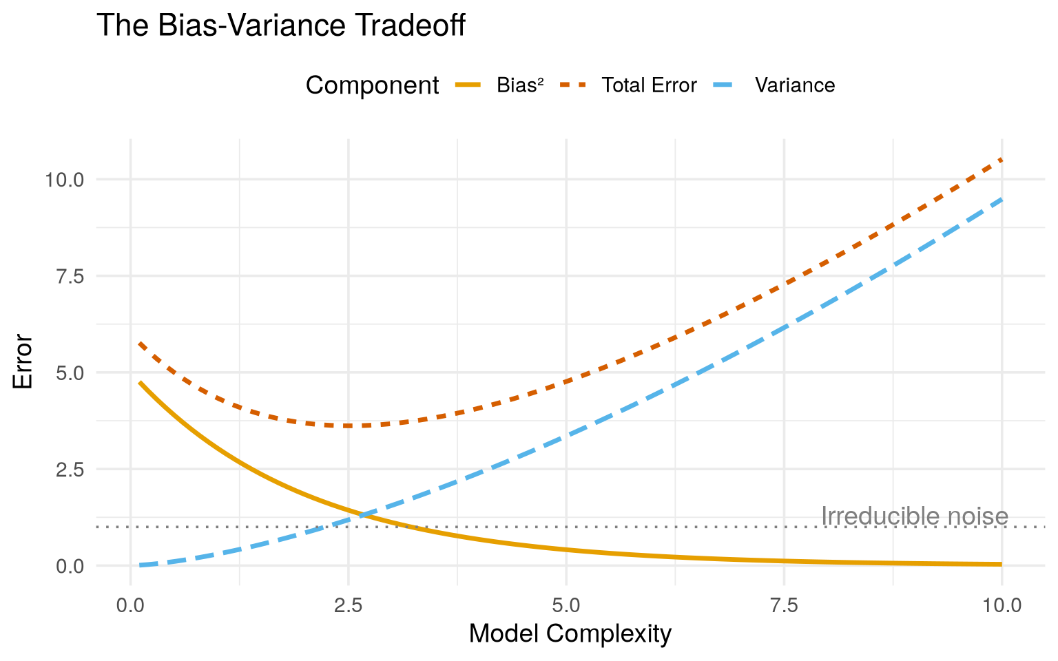
A core tenet of supervised learning is that the model is trained on a dataset that constitutes a sample of a (much) larger population. The model learns patterns from the training data, but its ultimate goal is to generalise to new, unseen data. This is where the concepts of bias and variance come into play.
12.4.1 The Bias-Variance Tradeoff
Every supervised model navigates a tension between two sources of error:
- Bias: Error from oversimplifying the model. A model with high bias misses important patterns. It underfits the data.
- Variance: Error from making the model too flexible. A model with high variance captures noise as if it were signal. It overfits the data.
The total prediction error can be decomposed as:
\[\text{Expected Error} = \text{Bias}^2 + \text{Variance} + \text{Irreducible Noise}\]
See this link for a derivation of this decomposition.
We can draw a clinical analogy to make this more concrete. Think of a diagnostic criterion:
- Too specific (high bias, low variance): A criterion that requires 5 out of 5 symptoms to diagnose a disease. It misses many true cases (underfitting — the rule is too rigid) but rarely triggers a false alarm.
- Too sensitive (low bias, high variance): A criterion that diagnoses the disease if any 1 of 5 symptoms is present. It catches nearly every true case but also flags many healthy individuals (overfitting to noise).
The optimal diagnostic criterion balances sensitivity and specificity. Similarly, the optimal ML model balances bias and variance.
Visualising the Tradeoff
TipYou have already seen bias and variance
In Chapter 4, you modelled non-linear relationships. A straight line through a U-shaped relationship has high bias — it systematically misses the true pattern. A spline with 20 knots that follows every wiggle in the training data has high variance — it captures noise and will perform poorly on new data. The bias-variance tradeoff is the formal name for this tension you have already experienced.
In practice, we cannot directly observe bias and variance separately. We detect the tradeoff by comparing training error (how well the model fits the data it learned from) and test error (how well it performs on new data). When training error is low but test error is high, the model is overfitting.
12.4.2 Training, Validation, and Test Sets
On what data should a model learn from? Since we want to strike the right balance between bias and variance, we need to evaluate the model on data it has not seen during learning. To that end, a recommended practice is to split the dataset into three parts: training, validation, and test sets.
Each set serves a distinct purpose.
| Set | Purpose | Typical Size |
|---|---|---|
| Training set | Fit the model (learn parameters) | 60–70% |
| Validation set | Tune hyperparameters, select among models | 15–20% |
| Test set | Final, unbiased performance estimate | 15–20% |
The most important methodological consideration in machine learning is that the test set must never be used for any decision — not for feature selection, not for hyperparameter tuning, not for choosing between models. It is opened exactly once, at the very end, to report final performance. If you use the test set to make modelling decisions, it becomes a validation set, and your reported performance will be optimistically biased.
WarningThe Cardinal Sin of Machine Learning
Using the test set during model development — and then reporting performance on that same test set — is the ML equivalent of p-hacking. It produces overoptimistic results that will not replicate. In clinical ML, this can mean deploying a model that performs worse in practice than expected, with potential patient harm.
Splitting data into training, validation, and test sets may be performed at random or in a stratified manner, but the key is that the splits are mutually exclusive. Potential pitfalls (also called data leakage) include:
- Repeated measurements from the same patient appearing in several splits.
- Site- or instrument-specific patterns in multi-centre data that correlate with the outcome, so the model learns institutional identity rather than biology.
- Features derived from information collected after the prediction time point (temporal leakage).
- Variables that exist as a consequence of the outcome rather than as independent predictors (e.g., a chemotherapy flag leaking a cancer diagnosis).
In clinical research, we often have hundreds (not millions) of patients. A single 70/15/15 split wastes data and produces unstable estimates. The solution is cross-validation.
12.4.3 Cross-Validation
Cross-validation (CV) is a resampling strategy that uses all the data for both training and validation, by rotating which portion is held out.
The most common approach is k-fold cross-validation:
- Randomly split the data into \(k\) equally sized folds (typically \(k = 5\) or \(k = 10\)).
- For each fold \(i = 1, \ldots, k\):
- Train the model on all folds except fold \(i\).
- Evaluate on fold \(i\).
- Average the \(k\) performance estimates.
This gives a more stable and less biased estimate of performance than a single train/test split. It is more stable because the estimate is an average over \(k\) different held-out sets rather than one arbitrary split, so a single unlucky partition can no longer dominate the result. It is less biased because every observation is used for validation exactly once and for training \(k-1\) times, so the model is trained on almost the full dataset each time — avoiding the pessimistic bias you get when a large chunk of data is permanently held out and never learned from.
Variants of Cross-Validation
Plain k-fold works well when the outcome is balanced and every row is an independent patient. Clinical data often violate those assumptions, so several variants exist. Each one fixes a specific problem you are likely to meet:
- Stratified k-fold: Ensures each fold has the same proportion of events/classes as the full dataset. Why it matters: with a rare outcome (say a 5% readmission rate and 10 folds), an ordinary random split could easily produce a fold with almost no events — giving a meaningless performance estimate for that fold. Stratification guarantees every fold contains a fair share of events. Use it by default for any classification problem.
- Repeated k-fold: Repeat the entire k-fold procedure \(m\) times with different random splits, then average. Why it matters: a single 10-fold split is itself somewhat random — shuffle the data differently and you get a slightly different performance estimate. Repeating (e.g. 10-fold repeated 5 times = 50 estimates) averages out that luck-of-the-draw and gives a more stable estimate.
- Leave-one-out (LOO): the extreme case where \(k = n\), so each fold is a single observation — the model is refit \(n\) times, each time leaving out one patient and predicting that patient. Why it behaves the way it does: because each training set contains almost all the data (\(n-1\) patients), the performance estimate is nearly unbiased. But the \(n\) held-out predictions are highly correlated (the training sets barely differ from one another), so averaging them removes little noise and the estimate has high variance — and refitting \(n\) times is computationally expensive. For these reasons LOO is worth it only for very small datasets, where you cannot afford to hold out 10% at a time.
- Grouped/clustered CV: When observations are not independent (e.g., multiple visits per patient, or patients clustered within hospitals), entire groups must be kept together — all of a patient’s rows go into the same fold. Why it matters: if the same patient appears in both the training and validation folds, the model can “recognise” them at validation time and post an inflated score that will not hold up on genuinely new patients. This is one of the most common and most damaging mistakes in clinical ML. Never split a patient’s data across training and validation sets.
Code
library(tidyverse)   # ggplot2 / dplyr / tibble
library(tidymodels)

# Simulate clinical data
set.seed(42)
n <- 500
clin_data <- tibble(
  age = rnorm(n, 60, 12),
  bmi = rnorm(n, 28, 5),
  sbp = rnorm(n, 135, 20),
  glucose = rnorm(n, 110, 30),
  smoking = rbinom(n, 1, 0.25),
  readmit = factor(
    rbinom(n, 1, 0.15),
    levels = c("0", "1"),
    labels = c("No", "Yes")
  )
)

# Create 10-fold CV with stratification
folds <- vfold_cv(clin_data, v = 10, strata = readmit, repeats = 5)
cat("Number of resamples:", nrow(folds), "\n")
cat("Training size per fold:", nrow(training(folds$splits[[1]])), "\n")
cat("Validation size per fold:", nrow(testing(folds$splits[[1]])), "\n")

# Fit logistic regression with cross-validation using tidymodels
log_spec <- logistic_reg() %>%
  set_engine("glm")

log_recipe <- recipe(readmit ~ ., data = clin_data)

log_wf <- workflow() %>%
  add_model(log_spec) %>%
  add_recipe(log_recipe)

cv_results <- fit_resamples(
  log_wf,
  resamples = folds,
  metrics = metric_set(roc_auc, accuracy)
)

collect_metrics(cv_results) |>
  knitr::kable(
    digits = 3,
    caption = "Cross-validated performance (mean +/- standard error across folds)."
  )
Number of resamples: 50
Training size per fold: 450
Validation size per fold: 50 | .metric | .estimator | mean | n | std_err | .config |
|---|---|---|---|---|---|
| accuracy | binary | 0.860 | 50 | 0.000 | pre0_mod0_post0 |
| roc_auc | binary | 0.466 | 50 | 0.017 | pre0_mod0_post0 |
Code
import numpy as np
import pandas as pd
from sklearn.model_selection import (StratifiedKFold, RepeatedStratifiedKFold,
                                      cross_val_score)
from sklearn.linear_model import LogisticRegression
from sklearn.preprocessing import StandardScaler
from sklearn.pipeline import make_pipeline

np.random.seed(42)
n = 500

X = pd.DataFrame({
    'age': np.random.normal(60, 12, n),
    'bmi': np.random.normal(28, 5, n),
    'sbp': np.random.normal(135, 20, n),
    'glucose': np.random.normal(110, 30, n),
    'smoking': np.random.binomial(1, 0.25, n)
})
y = np.random.binomial(1, 0.15, n)

# 10-fold stratified CV, repeated 5 times
cv = RepeatedStratifiedKFold(n_splits=10, n_repeats=5, random_state=42)

# Pipeline: scale features, then logistic regression
pipe = make_pipeline(StandardScaler(), LogisticRegression(max_iter=1000))

scores = cross_val_score(pipe, X, y, cv=cv, scoring='roc_auc')
print(f"Mean AUC: {scores.mean():.3f} (+/- {scores.std():.3f})")What the code is showing. This is a worked example of stratified, repeated cross-validation on simulated patient data. Walking through the output:
- It builds 10 folds and repeats the whole process 5 times, so it reports 50 train/validate cycles (
Number of resamples: 50). Each cycle trains the model on 90% of patients and checks it on the held-out 10%, with stratification keeping the event rate steady across folds. - The headline result is the mean AUC together with its spread (mean ± standard deviation). The mean is your best single estimate of how well the model discriminates; the spread tells you how much that estimate wobbles depending on which patients land in which fold. A tight spread means the estimate is trustworthy; a wide spread is a warning that performance is fragile, often a sign of too little data.
The point of the exercise is not the specific number (the data are random here, so the AUC will sit near 0.5) but the workflow: this is the template you reuse for real data, simply swapping in your own dataset and model.
12.4.4 Feature Engineering in Clinical Data
Feature engineering is the process of transforming raw variables into features that are more useful for modelling. In clinical ML, this often means incorporating domain knowledge.
Examples of Clinical Feature Engineering
| Raw Data | Engineered Feature | Rationale |
|---|---|---|
| Date of birth + visit date | Age at visit | More meaningful than raw dates |
| Systolic BP, Diastolic BP | Mean arterial pressure, pulse pressure | Physiologically meaningful composites |
| Serum creatinine, age, sex, race | eGFR (CKD-EPI equation) | Standard clinical measure of kidney function |
| Multiple lab values over time | Rate of change (slope), variability (SD) | Trajectory matters more than single values |
| ICD-10 codes | Charlson comorbidity index | Summarises comorbidity burden |
| Free-text clinical notes | Extracted symptoms via natural language processing (NLP) | Unlocks unstructured data |
| Medication list | Binary flags for drug classes | Captures treatment intent |
TipDomain Knowledge Is Your Superpower
Clinical researchers have a massive advantage in ML: you understand the data. A computer scientist might feed raw creatinine into a model; you know to compute eGFR. A data scientist might treat blood pressure as two independent numbers; you know that pulse pressure has specific physiological meaning. Feature engineering is where clinical expertise directly improves model performance.
12.4.5 Feature Selection
With electronic health record data, you might have hundreds or thousands of candidate features. Including all of them risks overfitting and reduces interpretability. Feature selection identifies the most informative subset. Three common approaches are:
1. Filter methods: Rank features by some statistical criterion (correlation with outcome, mutual information, chi-squared test) before fitting any model. Fast but ignores feature interactions.
2. Wrapper methods: Iteratively fit models with different feature subsets and select the best-performing set. Examples: forward selection, backward elimination, recursive feature elimination (RFE). More accurate but computationally expensive.
3. Embedded methods: Feature selection happens as part of model fitting. Examples: LASSO regression (L1 penalty shrinks some coefficients to zero), random forest variable importance, elastic net. Often the best practical choice.
Code
library(tidyverse)   # ggplot2 / dplyr / tibble
library(tidymodels)

# LASSO for feature selection
set.seed(42)
n <- 400
df_feat <- tibble(
  age = rnorm(n, 60, 12),
  bmi = rnorm(n, 28, 5),
  sbp = rnorm(n, 135, 20),
  glucose = rnorm(n, 110, 30),
  smoking = rbinom(n, 1, 0.25),
  noise1 = rnorm(n), # irrelevant
  noise2 = rnorm(n), # irrelevant
  noise3 = rnorm(n), # irrelevant
  outcome = factor(
    rbinom(n, 1, plogis(-3 + 0.02 * age + 0.05 * bmi)),
    labels = c("No", "Yes")
  )
)

# LASSO logistic regression
lasso_spec <- logistic_reg(penalty = 0.01, mixture = 1) %>%
  set_engine("glmnet")

lasso_recipe <- recipe(outcome ~ ., data = df_feat) %>%
  step_normalize(all_numeric_predictors())

lasso_wf <- workflow() %>%
  add_model(lasso_spec) %>%
  add_recipe(lasso_recipe)

lasso_fit <- fit(lasso_wf, data = df_feat)

# Extract coefficients
tidy(lasso_fit) %>%
  filter(term != "(Intercept)") %>%
  arrange(desc(abs(estimate))) %>%
  knitr::kable(
    digits = 3,
    caption = "LASSO coefficients, ordered by absolute size (variables shrunk to zero are dropped)."
)| term | estimate | penalty |
|---|---|---|
| age | 0.275 | 0.01 |
| smoking | 0.250 | 0.01 |
| bmi | 0.152 | 0.01 |
| sbp | 0.136 | 0.01 |
| noise2 | -0.134 | 0.01 |
| noise1 | 0.088 | 0.01 |
| noise3 | -0.077 | 0.01 |
| glucose | 0.025 | 0.01 |
Code
from sklearn.linear_model import LogisticRegression
from sklearn.feature_selection import RFE
from sklearn.preprocessing import StandardScaler
import pandas as pd
import numpy as np

np.random.seed(42)
n = 400
X = pd.DataFrame({
    'age': np.random.normal(60, 12, n),
    'bmi': np.random.normal(28, 5, n),
    'sbp': np.random.normal(135, 20, n),
    'glucose': np.random.normal(110, 30, n),
    'smoking': np.random.binomial(1, 0.25, n),
    'noise1': np.random.normal(0, 1, n),
    'noise2': np.random.normal(0, 1, n),
    'noise3': np.random.normal(0, 1, n)
})
y = np.random.binomial(1, 1 / (1 + np.exp(-(-3 + 0.02 * X['age'] + 0.05 * X['bmi']))))

# LASSO feature selection
scaler = StandardScaler()
X_scaled = scaler.fit_transform(X)

lasso = LogisticRegression(penalty='l1', solver='saga', C=1.0, max_iter=5000)
lasso.fit(X_scaled, y)

coef_df = pd.DataFrame({
    'Feature': X.columns,
    'Coefficient': lasso.coef_[0]
}).sort_values('Coefficient', key=abs, ascending=False)

print("LASSO Coefficients (features with 0 coefficient are excluded):")
print(coef_df.to_string(index=False))

# Recursive Feature Elimination
rfe = RFE(LogisticRegression(max_iter=5000), n_features_to_select=4)
rfe.fit(X_scaled, y)
selected = X.columns[rfe.support_]
print(f"\nRFE selected features: {list(selected)}")
LogisticRegression(max_iter=5000, penalty='l1', solver='saga')In a Jupyter environment, please rerun this cell to show the HTML representation or trust the notebook.
On GitHub, the HTML representation is unable to render, please try loading this page with nbviewer.org.
Parameters
Fitted attributes
LASSO Coefficients (features with 0 coefficient are excluded):
Feature  Coefficient
    age     0.219566
    bmi     0.204396
 noise1    -0.176441
smoking    -0.161687
 noise3     0.136270
    sbp     0.060393
 noise2     0.020577
glucose     0.000000
RFE(estimator=LogisticRegression(max_iter=5000), n_features_to_select=4)In a Jupyter environment, please rerun this cell to show the HTML representation or trust the notebook.
On GitHub, the HTML representation is unable to render, please try loading this page with nbviewer.org.
Parameters
Fitted attributes
| Name | Type | Value |
|---|---|---|
| classes_ classes_: ndarray of shape (n_classes,) The classes labels. Only available when `estimator` is a classifier. |
ndarray[int64](2,) | [0,1] |
| estimator_ estimator_: ``Estimator`` instance The fitted estimator used to select features. |
LogisticRegression | LogisticRegre...max_iter=5000) |
| n_features_ n_features_: int The number of selected features. |
int64 | np.int64(4) |
| n_features_in_ n_features_in_: int Number of features seen during :term:`fit`. Only defined if the underlying estimator exposes such an attribute when fit. .. versionadded:: 0.24 |
int | 8 |
| ranking_ ranking_: ndarray of shape (n_features,) The feature ranking, such that ``ranking_[i]`` corresponds to the ranking position of the i-th feature. Selected (i.e., estimated best) features are assigned rank 1. |
ndarray[int64](8,) | [1,1,3,...,1,4,2] |
| support_ support_: ndarray of shape (n_features,) The mask of selected features. |
ndarray[bool](8,) | [ True, True,False,..., True,False,False] |
LogisticRegression(max_iter=5000)
Parameters
4 features
| x0 |
| x1 |
| x4 |
| x5 |
RFE selected features: ['age', 'bmi', 'smoking', 'noise1']What the code is telling you. Both examples are a small experiment: we built a dataset where age and bmi genuinely relate to the outcome, while noise1, noise2, and noise3 are pure random noise that we added on purpose. A good feature-selection method should keep the real predictors and discard the noise. That is exactly what you should see in the output:
- The LASSO table lists each predictor with its coefficient, sorted by size. The L1 penalty shrinks unhelpful coefficients all the way to exactly zero — so the noise variables drop out (coefficient = 0) while age and BMI survive with non-zero coefficients. Reading the table top-to-bottom tells you which variables the model considers most important.
- The RFE line prints the handful of features it chose to keep; the noise variables should not be among them.
The clinical point is reassurance: when you face a spreadsheet with dozens of candidate variables, these methods let the data tell you which ones carry signal, rather than you guessing or keeping everything (which invites overfitting). If a variable you expected to matter gets dropped, that is itself informative and worth investigating.
12.5 ML vs Traditional Statistics: What Is Actually Different?
This is a question clinical researchers often ask, and the honest answer is: less than you think.
| Aspect | Traditional Statistics | Machine Learning |
|---|---|---|
| Primary goal | Inference (understand relationships) | Prediction (forecast accurately) |
| Model choice | Guided by theory and assumptions | Guided by cross-validated performance |
| Feature selection | Guided by domain knowledge, parsimony | Data-driven, automated |
| Evaluation | p-values, confidence intervals | AUC, accuracy, calibration, cross-validation |
| Interpretability | Usually high (coefficients) | Varies (logistic regression = high; deep learning = low) |
| Sample size | Can work with small samples | Often needs more data for complex models |
| Assumptions | Explicit (linearity, normality, etc.) | Implicit (representative data, stationarity) |
The biggest practical difference is in workflow. Statistical modelling typically follows a hypothesis-driven process: specify a model based on theory, fit it, check assumptions, interpret coefficients. ML follows a more empirical process: try many models, tune them, evaluate on held-out data, pick the best performer.
Neither approach is inherently superior. For a clinical trial with 200 patients and 5 pre-specified predictors, logistic regression is perfectly appropriate and more interpretable than a random forest. For a hospital system with 500,000 patient records, 1,000 candidate features, and the goal of predicting ICU transfer, a gradient-boosted tree with cross-validated tuning may outperform logistic regression.
12.6 Exercises
TipExercise 1: Feature Engineering and Cross-Validation
Using the simulated clinical dataset below, compare two logistic regression models using 10-fold stratified cross-validation:
- Model A (raw features): Fit logistic regression on the raw variables as given.
- Model B (engineered features): Add clinically motivated features — e.g., eGFR estimated from creatinine, age, and sex; a hemoglobin-to-platelet ratio; log-transformed WBC — and fit logistic regression on the expanded feature set.
Report AUC for both models. Does feature engineering improve performance? Why or why not?
Code
library(tidyverse) # tibble()
library(tidymodels) # vfold_cv(), logistic_reg(), recipe(), etc.

set.seed(123)
n <- 600
ex_data <- tibble(
  age = rnorm(n, 65, 10),
  sex = rbinom(n, 1, 0.5),
  creatinine = rlnorm(n, 0, 0.5),
  hemoglobin = rnorm(n, 12, 2),
  platelets = rnorm(n, 250, 70),
  wbc = rlnorm(n, 2, 0.4),
  icu = factor(
    rbinom(
      n,
      1,
      plogis(-4 + 0.03 * age + 0.5 * creatinine)
    ),
    labels = c("No", "Yes")
  )
)

# Your code:
# 1. Create two recipes: one with raw features, one adding engineered features
#    (e.g., step_mutate to add eGFR, hb/platelet ratio, log(wbc))
# 2. Set up logistic_reg() workflows for both
# 3. Use vfold_cv with strata = icu
# 4. Compare using roc_auc
Code
import numpy as np
import pandas as pd
from sklearn.linear_model import LogisticRegression
from sklearn.model_selection import cross_val_score, StratifiedKFold
from sklearn.preprocessing import StandardScaler
from sklearn.pipeline import make_pipeline

np.random.seed(123)
n = 600

# Your code:
# 1. Create X with raw features (age, sex, creatinine, hemoglobin, platelets, wbc)
# 2. Create X_eng with additional engineered features
#    (e.g., eGFR from creatinine/age/sex, hb/platelet ratio, log(wbc))
# 3. Generate y from age and creatinine
# 4. Compare LogisticRegression on X vs X_eng using cross_val_score
#    with scoring='roc_auc'
NoteSolution
Code
# =============================================================================
# Chapter 7, Exercise 1: Feature Engineering and Cross-Validation
# Compare logistic regression with raw features vs engineered features
# using 10-fold stratified CV. Report AUC for both models.
# =============================================================================

library(tidyverse)
library(tidymodels)

# --- Simulate the clinical dataset ---
set.seed(123)
n <- 600
ex_data <- tibble(
  age = rnorm(n, 65, 10),
  sex = rbinom(n, 1, 0.5),
  creatinine = rlnorm(n, 0, 0.5),
  hemoglobin = rnorm(n, 12, 2),
  platelets = rnorm(n, 250, 70),
  wbc = rlnorm(n, 2, 0.4),
  icu = factor(
    rbinom(n, 1, plogis(-4 + 0.03 * age + 0.5 * creatinine)),
    labels = c("No", "Yes")
  )
)

cat("ICU admission rate:", mean(ex_data$icu == "Yes"), "\n")

# --- 10-fold stratified cross-validation ---
set.seed(42)
folds <- vfold_cv(ex_data, v = 10, strata = icu)

# --- Model A: raw features ---
raw_recipe <- recipe(icu ~ ., data = ex_data) %>%
  step_normalize(all_numeric_predictors())

lr_spec <- logistic_reg() %>%
  set_engine("glm")

raw_wf <- workflow() %>%
  add_model(lr_spec) %>%
  add_recipe(raw_recipe)

raw_results <- fit_resamples(raw_wf, resamples = folds,
                             metrics = metric_set(roc_auc))

# --- Model B: engineered features ---
eng_recipe <- recipe(icu ~ ., data = ex_data) %>%
  step_mutate(
    # Simplified eGFR (CKD-EPI-inspired, not the full equation)
    egfr = 140 *
      (pmin(creatinine, 0.9) / 0.9)^(-0.411) *
      (pmax(creatinine, 0.9) / 0.9)^(-1.209) *
      0.993^age *
      ifelse(sex == 1, 1.0, 1.018),
    # Hemoglobin-to-platelet ratio
    hb_platelet_ratio = hemoglobin / platelets,
    # Log-transformed WBC (reduces skew)
    log_wbc = log(wbc)
  ) %>%
  step_normalize(all_numeric_predictors())

eng_wf <- workflow() %>%
  add_model(lr_spec) %>%
  add_recipe(eng_recipe)

eng_results <- fit_resamples(eng_wf, resamples = folds,
                             metrics = metric_set(roc_auc))

# --- Collect and compare results ---
raw_metrics <- collect_metrics(raw_results) %>% mutate(model = "A (raw)")
eng_metrics <- collect_metrics(eng_results) %>% mutate(model = "B (engineered)")

comparison <- bind_rows(raw_metrics, eng_metrics) %>%
  select(model, .metric, mean, std_err)

print(comparison)

# --- Interpretation ---
# In this simulated dataset the true outcome depends on age and creatinine
# via a logistic link. Since logistic regression can already capture that
# linear relationship from the raw features, the engineered features (eGFR,
# ratios, log transforms) may add only a modest improvement — or none at all.
#
# In real clinical data, feature engineering often matters more: eGFR is a
# non-linear transform of creatinine that better reflects kidney function,
# and log-WBC handles the right skew common in lab values. The lesson is
# that engineered features encode domain knowledge the model cannot discover
# on its own from raw inputs — even if the benefit is small in this toy
# example.
Code
# =============================================================================
# Chapter 7, Exercise 1: Feature Engineering and Cross-Validation
# Compare logistic regression with raw features vs engineered features
# using 10-fold stratified CV. Report AUC for both models.
# =============================================================================

import numpy as np
import pandas as pd
from sklearn.linear_model import LogisticRegression
from sklearn.model_selection import cross_val_score, StratifiedKFold
from sklearn.preprocessing import StandardScaler
from sklearn.pipeline import make_pipeline

# --- Simulate the clinical dataset ---
np.random.seed(123)
n = 600

X = pd.DataFrame({
    'age': np.random.normal(65, 10, n),
    'sex': np.random.binomial(1, 0.5, n),
    'creatinine': np.random.lognormal(0, 0.5, n),
    'hemoglobin': np.random.normal(12, 2, n),
    'platelets': np.random.normal(250, 70, n),
    'wbc': np.random.lognormal(2, 0.4, n)
})

y = np.random.binomial(
    1,
    1 / (1 + np.exp(-(-4 + 0.03 * X['age'] + 0.5 * X['creatinine'])))
)
print(f"ICU admission rate: {y.mean():.3f}")

# --- 10-fold stratified CV ---
cv = StratifiedKFold(n_splits=10, shuffle=True, random_state=42)

# --- Model A: raw features ---
pipe_raw = make_pipeline(StandardScaler(), LogisticRegression(max_iter=1000))
scores_raw = cross_val_score(pipe_raw, X, y, cv=cv, scoring='roc_auc')
print(f"\nModel A (raw features) AUC: {scores_raw.mean():.3f} (+/- {scores_raw.std():.3f})")

# --- Model B: engineered features ---
X_eng = X.copy()

# Simplified eGFR (CKD-EPI-inspired, not the full equation)
# Higher creatinine -> lower eGFR; older age -> lower eGFR
X_eng['egfr'] = (
    140 * (np.minimum(X['creatinine'], 0.9) / 0.9) ** (-0.411)
    * (np.maximum(X['creatinine'], 0.9) / 0.9) ** (-1.209)
    * 0.993 ** X['age']
    * np.where(X['sex'] == 1, 1.0, 1.018)
)

# Hemoglobin-to-platelet ratio
X_eng['hb_platelet_ratio'] = X['hemoglobin'] / X['platelets']

# Log-transformed WBC (reduces skew)
X_eng['log_wbc'] = np.log(X['wbc'])

pipe_eng = make_pipeline(StandardScaler(), LogisticRegression(max_iter=1000))
scores_eng = cross_val_score(pipe_eng, X_eng, y, cv=cv, scoring='roc_auc')
print(f"Model B (engineered)   AUC: {scores_eng.mean():.3f} (+/- {scores_eng.std():.3f})")

# --- Comparison ---
results = pd.DataFrame({
    'Model': ['A (raw)', 'B (engineered)'],
    'Mean AUC': [scores_raw.mean(), scores_eng.mean()],
    'Std AUC': [scores_raw.std(), scores_eng.std()]
})
print("\n", results.to_string(index=False))

# --- Interpretation ---
# In this simulated dataset the true outcome depends on age and creatinine
# via a logistic link. Since logistic regression can already capture that
# linear relationship from the raw features, the engineered features (eGFR,
# ratios, log transforms) may add only a modest improvement — or none at all.
#
# In real clinical data, feature engineering often matters more: eGFR is a
# non-linear transform of creatinine that better reflects kidney function,
# and log-WBC handles the right skew common in lab values. The lesson is
# that engineered features encode domain knowledge the model cannot discover
# on its own from raw inputs — even if the benefit is small in this toy
# example.
TipExercise 2: Feature Engineering Challenge
You have the following raw variables for a diabetes prediction model:
height_cm,weight_kgsbp,dbp(systolic and diastolic blood pressure)fasting_glucose,hba1cage,sexwaist_circumference,hip_circumferencetotal_cholesterol,hdl,ldl,triglycerides
- List at least 5 clinically meaningful engineered features you could create from these variables. For each, explain why it is clinically meaningful.
- Implement the feature engineering in R (using
recipes) or Python (using pandas/sklearn). - Discuss which original features might become redundant after engineering.
NoteSolution
Code
# =============================================================================
# Chapter 7, Exercise 2: Feature Engineering Challenge
# Engineer clinically meaningful features from raw variables for a diabetes
# prediction model. Implement using tidymodels recipes.
# =============================================================================

library(tidyverse)
library(tidymodels)

# --- Simulate raw clinical data ---
set.seed(42)
n <- 500

raw_data <- tibble(
  height_cm = rnorm(n, 170, 10),
  weight_kg = rnorm(n, 80, 15),
  sbp = rnorm(n, 130, 18),
  dbp = rnorm(n, 82, 12),
  fasting_glucose = rnorm(n, 105, 25),
  hba1c = rnorm(n, 5.8, 0.8),
  age = rnorm(n, 55, 12),
  sex = sample(c("Male", "Female"), n, replace = TRUE),
  waist_circumference = rnorm(n, 95, 12),
  hip_circumference = rnorm(n, 100, 10),
  total_cholesterol = rnorm(n, 200, 40),
  hdl = rnorm(n, 50, 15),
  ldl = rnorm(n, 120, 35),
  triglycerides = rnorm(n, 150, 60),
  diabetes = factor(rbinom(n, 1, 0.3), labels = c("No", "Yes"))
)

# --- Part 1: Clinically meaningful engineered features ---
# 1. BMI = weight_kg / (height_m)^2
#    WHY: Standard obesity measure; strong risk factor for Type 2 diabetes.
#
# 2. Pulse Pressure = sbp - dbp
#    WHY: Reflects arterial stiffness; associated with cardiovascular risk
#         and metabolic syndrome.
#
# 3. Mean Arterial Pressure (MAP) = dbp + (sbp - dbp) / 3
#    WHY: Measures average perfusion pressure; linked to vascular health.
#
# 4. Waist-to-Hip Ratio (WHR) = waist_circumference / hip_circumference
#    WHY: Central adiposity is a stronger predictor of insulin resistance
#         than BMI alone.
#
# 5. Non-HDL Cholesterol = total_cholesterol - hdl
#    WHY: Captures all atherogenic lipoproteins; recommended by guidelines
#         as a secondary target in diabetes management.
#
# 6. Triglyceride-to-HDL Ratio = triglycerides / hdl
#    WHY: A proxy for insulin resistance; high TG/HDL ratio is associated
#         with increased diabetes risk.
#
# 7. LDL/HDL Ratio = ldl / hdl
#    WHY: Captures atherogenic dyslipidemia profile common in diabetes.

# --- Part 2: Implement feature engineering with recipes ---
diabetes_recipe <- recipe(diabetes ~ ., data = raw_data) %>%
  # BMI: weight / height_m^2
  step_mutate(
    height_m = height_cm / 100,
    bmi = weight_kg / height_m^2,
    # Pulse pressure
    pulse_pressure = sbp - dbp,
    # Mean arterial pressure
    map = dbp + (sbp - dbp) / 3,
    # Waist-to-hip ratio
    whr = waist_circumference / hip_circumference,
    # Non-HDL cholesterol
    non_hdl = total_cholesterol - hdl,
    # Triglyceride-to-HDL ratio
    tg_hdl_ratio = triglycerides / hdl,
    # LDL/HDL ratio
    ldl_hdl_ratio = ldl / hdl
  ) %>%
  # Remove intermediate and redundant variables
  step_rm(height_m) %>%
  step_normalize(all_numeric_predictors()) %>%
  step_dummy(all_nominal_predictors())

# Prepare (bake) the recipe to see the result
prepped <- prep(diabetes_recipe)
engineered_data <- bake(prepped, new_data = NULL)

cat("Original variables:", ncol(raw_data) - 1, "\n")
cat("Engineered dataset columns:", ncol(engineered_data) - 1, "\n")
cat("\nColumn names:\n")
print(names(engineered_data))

# --- Part 3: Discuss redundant features ---
# After engineering:
# - height_cm and weight_kg may become redundant once BMI is computed
#   (though height or weight alone may still carry predictive signal).
# - sbp and dbp are partially captured by pulse_pressure and MAP,
#   though keeping them may still be useful for tree-based models.
# - waist_circumference and hip_circumference are largely captured by WHR.
# - total_cholesterol is partly captured by non_hdl (since non_hdl = TC - HDL).
# - Individual lipids (hdl, ldl, triglycerides) overlap with the ratios,
#   but a LASSO or tree model can sort out which representation is most useful.
#
# In practice, include both raw and engineered features and let a
# regularised model (LASSO, elastic net) or tree-based model perform
# implicit feature selection.
Code
# =============================================================================
# Chapter 7, Exercise 2: Feature Engineering Challenge
# Engineer clinically meaningful features from raw variables for a diabetes
# prediction model. Implement using pandas and sklearn.
# =============================================================================

import numpy as np
import pandas as pd
from sklearn.preprocessing import StandardScaler

# --- Simulate raw clinical data ---
np.random.seed(42)
n = 500

raw_data = pd.DataFrame({
    'height_cm': np.random.normal(170, 10, n),
    'weight_kg': np.random.normal(80, 15, n),
    'sbp': np.random.normal(130, 18, n),
    'dbp': np.random.normal(82, 12, n),
    'fasting_glucose': np.random.normal(105, 25, n),
    'hba1c': np.random.normal(5.8, 0.8, n),
    'age': np.random.normal(55, 12, n),
    'sex': np.random.choice(['Male', 'Female'], n),
    'waist_circumference': np.random.normal(95, 12, n),
    'hip_circumference': np.random.normal(100, 10, n),
    'total_cholesterol': np.random.normal(200, 40, n),
    'hdl': np.random.normal(50, 15, n),
    'ldl': np.random.normal(120, 35, n),
    'triglycerides': np.random.normal(150, 60, n),
})
y = np.random.binomial(1, 0.3, n)

# --- Part 1: Clinically meaningful engineered features ---
# 1. BMI = weight_kg / (height_m)^2
#    WHY: Standard obesity measure; strong risk factor for Type 2 diabetes.
#
# 2. Pulse Pressure = sbp - dbp
#    WHY: Reflects arterial stiffness; associated with cardiovascular risk
#         and metabolic syndrome.
#
# 3. Mean Arterial Pressure (MAP) = dbp + (sbp - dbp) / 3
#    WHY: Measures average perfusion pressure; linked to vascular health.
#
# 4. Waist-to-Hip Ratio (WHR) = waist / hip
#    WHY: Central adiposity is a stronger predictor of insulin resistance
#         than BMI alone.
#
# 5. Non-HDL Cholesterol = total_cholesterol - hdl
#    WHY: Captures all atherogenic lipoproteins; recommended by guidelines
#         as a secondary target in diabetes management.
#
# 6. Triglyceride-to-HDL Ratio = triglycerides / hdl
#    WHY: A proxy for insulin resistance; high TG/HDL ratio is associated
#         with increased diabetes risk.
#
# 7. LDL/HDL Ratio = ldl / hdl
#    WHY: Captures atherogenic dyslipidemia profile common in diabetes.

# --- Part 2: Implement feature engineering ---
df = raw_data.copy()

# Compute engineered features
df['bmi'] = df['weight_kg'] / (df['height_cm'] / 100) ** 2
df['pulse_pressure'] = df['sbp'] - df['dbp']
df['map'] = df['dbp'] + (df['sbp'] - df['dbp']) / 3
df['whr'] = df['waist_circumference'] / df['hip_circumference']
df['non_hdl'] = df['total_cholesterol'] - df['hdl']
df['tg_hdl_ratio'] = df['triglycerides'] / df['hdl']
df['ldl_hdl_ratio'] = df['ldl'] / df['hdl']

# Encode sex as binary
df['sex_male'] = (df['sex'] == 'Male').astype(int)
df = df.drop(columns=['sex'])

print(f"Original features: {raw_data.shape[1]}")
print(f"Engineered features: {df.shape[1]}")
print(f"\nColumn names:\n{list(df.columns)}")

# Scale numeric features
scaler = StandardScaler()
numeric_cols = df.select_dtypes(include=[np.number]).columns
df_scaled = df.copy()
df_scaled[numeric_cols] = scaler.fit_transform(df[numeric_cols])

print(f"\nFirst few rows of engineered data:")
print(df_scaled.head())

# --- Part 3: Discuss redundant features ---
# After engineering:
# - height_cm and weight_kg may become redundant once BMI is computed
#   (though they may still carry independent predictive signal).
# - sbp and dbp are partially captured by pulse_pressure and MAP,
#   though keeping them may still be useful for tree-based models.
# - waist_circumference and hip_circumference are largely captured by WHR.
# - total_cholesterol is partly captured by non_hdl (since non_hdl = TC - HDL).
# - Individual lipids (hdl, ldl, triglycerides) overlap with the ratios,
#   but a LASSO or tree model can sort out which representation is most useful.
#
# In practice, include both raw and engineered features and let a
# regularised model (LASSO, elastic net) or tree-based model perform
# implicit feature selection.
TipExercise 3: The Bias-Variance Tradeoff in Practice
Using polynomial regression on a simulated dataset:
- Fit polynomials of degree 1, 3, 5, 10, and 20 to a training set.
- Plot the fitted curves overlaid on the data.
- Compute training error and test error for each degree.
- Identify the degree that minimises test error. Explain this in terms of the bias-variance tradeoff.
Code
import numpy as np
from sklearn.preprocessing import PolynomialFeatures
from sklearn.linear_model import LinearRegression
from sklearn.metrics import mean_squared_error

np.random.seed(42)
x_train = np.sort(np.random.uniform(0, 10, 50))
y_train = np.sin(x_train) + np.random.normal(0, 0.3, 50)
x_test = np.sort(np.random.uniform(0, 10, 200))
y_test = np.sin(x_test) + np.random.normal(0, 0.3, 200)

# Your code: loop over degrees [1, 3, 5, 10, 20]
# Fit PolynomialFeatures + LinearRegression
# Compute train and test RMSE
NoteSolution
Code
# =============================================================================
# Chapter 7, Exercise 3: The Bias-Variance Tradeoff in Practice
# Fit polynomials of degree 1, 3, 5, 10, and 20 to a training set.
# Plot fitted curves, compute training/test error, identify optimal degree.
# =============================================================================

library(tidyverse)

# --- Generate data ---
set.seed(42)
x_train <- sort(runif(50, 0, 10))
y_train <- sin(x_train) + rnorm(50, 0, 0.3)
x_test <- sort(runif(200, 0, 10))
y_test <- sin(x_test) + rnorm(200, 0, 0.3)

train_df <- tibble(x = x_train, y = y_train)
test_df  <- tibble(x = x_test,  y = y_test)

# --- Fit polynomials and compute RMSE ---
degrees <- c(1, 3, 5, 10, 20)
results <- tibble(degree = integer(), train_rmse = double(), test_rmse = double())

# Also store predictions for plotting
plot_data <- tibble()

for (d in degrees) {
  # Fit polynomial of degree d
  fit <- lm(y ~ poly(x, degree = d, raw = TRUE), data = train_df)

  # Predictions on train and test
  pred_train <- predict(fit, newdata = train_df)
  pred_test  <- predict(fit, newdata = test_df)

  # Compute RMSE
  rmse_train <- sqrt(mean((y_train - pred_train)^2))
  rmse_test  <- sqrt(mean((y_test - pred_test)^2))

  results <- bind_rows(results,
                       tibble(degree = d, train_rmse = rmse_train, test_rmse = rmse_test))

  # Smooth curve for plotting
  x_grid <- seq(0, 10, length.out = 300)
  pred_grid <- predict(fit, newdata = tibble(x = x_grid))
  # Clip extreme predictions for high-degree polynomials
  pred_grid <- pmin(pmax(pred_grid, -3), 3)
  plot_data <- bind_rows(plot_data,
                         tibble(x = x_grid, y_pred = pred_grid,
                                degree = paste("Degree", d)))
}

# --- Print RMSE results ---
cat("Polynomial Regression: Training vs Test RMSE\n")
cat("=============================================\n")
print(results)

# --- Part 2: Plot fitted curves ---
p1 <- ggplot() +
  geom_point(data = train_df, aes(x, y), alpha = 0.5, size = 2) +
  geom_line(data = plot_data, aes(x, y_pred, color = degree), linewidth = 1) +
  geom_line(data = tibble(x = seq(0, 10, 0.01), y = sin(seq(0, 10, 0.01))),
            aes(x, y), linetype = "dashed", color = "black", linewidth = 0.8) +
  labs(title = "Polynomial Fits of Varying Complexity",
       subtitle = "Dashed line = true function sin(x)",
       x = "x", y = "y", color = "Polynomial") +
  theme_minimal(base_size = 14) +
  theme(legend.position = "top")

print(p1)

# --- Part 3: Plot training vs test error ---
results_long <- results %>%
  pivot_longer(cols = c(train_rmse, test_rmse),
               names_to = "set", values_to = "rmse") %>%
  mutate(set = ifelse(set == "train_rmse", "Training", "Test"))

p2 <- ggplot(results_long, aes(x = degree, y = rmse, color = set)) +
  geom_line(linewidth = 1.2) +
  geom_point(size = 3) +
  labs(title = "Training vs Test RMSE by Polynomial Degree",
       x = "Polynomial Degree", y = "RMSE", color = "Dataset") +
  theme_minimal(base_size = 14) +
  theme(legend.position = "top")

print(p2)

# --- Part 4: Interpretation ---
best_degree <- results$degree[which.min(results$test_rmse)]
cat("\nBest polynomial degree (lowest test RMSE):", best_degree, "\n")
cat("\nInterpretation (Bias-Variance Tradeoff):\n")
cat("- Degree 1 (linear): High bias -- too simple to capture the sine curve.\n")
cat("  Underfits both training and test data.\n")
cat("- Degree 3-5: Good balance. Captures the main curvature of sin(x)\n")
cat("  without fitting noise. Test error is minimized here.\n")
cat("- Degree 10-20: High variance -- the polynomial wiggles to fit\n")
cat("  training noise. Training error drops but test error increases.\n")
cat("  This is classic overfitting.\n")
cat("\nThe optimal degree (~3-5) sits at the sweet spot of the bias-variance\n")
cat("tradeoff, where the model is flexible enough to capture the true\n")
cat("pattern but not so flexible that it memorizes noise.\n")
Code
# =============================================================================
# Chapter 7, Exercise 3: The Bias-Variance Tradeoff in Practice
# Fit polynomials of degree 1, 3, 5, 10, and 20 to a training set.
# Plot fitted curves, compute training/test error, identify optimal degree.
# =============================================================================

import numpy as np
import matplotlib.pyplot as plt
from sklearn.preprocessing import PolynomialFeatures
from sklearn.linear_model import LinearRegression
from sklearn.metrics import mean_squared_error

# --- Generate data ---
np.random.seed(42)
x_train = np.sort(np.random.uniform(0, 10, 50))
y_train = np.sin(x_train) + np.random.normal(0, 0.3, 50)
x_test = np.sort(np.random.uniform(0, 10, 200))
y_test = np.sin(x_test) + np.random.normal(0, 0.3, 200)

# --- Fit polynomials and compute RMSE ---
degrees = [1, 3, 5, 10, 20]
results = []
predictions = {}

for d in degrees:
    # Create polynomial features and fit
    poly = PolynomialFeatures(degree=d, include_bias=False)
    X_train_poly = poly.fit_transform(x_train.reshape(-1, 1))
    X_test_poly = poly.transform(x_test.reshape(-1, 1))

    model = LinearRegression()
    model.fit(X_train_poly, y_train)

    # Predictions
    pred_train = model.predict(X_train_poly)
    pred_test = model.predict(X_test_poly)

    # RMSE
    rmse_train = np.sqrt(mean_squared_error(y_train, pred_train))
    rmse_test = np.sqrt(mean_squared_error(y_test, pred_test))

    results.append({'degree': d, 'train_rmse': rmse_train, 'test_rmse': rmse_test})

    # Smooth curve for plotting
    x_grid = np.linspace(0, 10, 300).reshape(-1, 1)
    X_grid_poly = poly.transform(x_grid)
    pred_grid = model.predict(X_grid_poly)
    # Clip extreme predictions for high-degree polynomials
    pred_grid = np.clip(pred_grid, -3, 3)
    predictions[d] = (x_grid.ravel(), pred_grid)

# --- Print RMSE results ---
print("Polynomial Regression: Training vs Test RMSE")
print("=" * 50)
print(f"{'Degree':>8s}  {'Train RMSE':>12s}  {'Test RMSE':>12s}")
print("-" * 50)
for r in results:
    print(f"{r['degree']:>8d}  {r['train_rmse']:>12.4f}  {r['test_rmse']:>12.4f}")

# --- Part 2: Plot fitted curves ---
fig, ax = plt.subplots(figsize=(10, 6))
ax.scatter(x_train, y_train, alpha=0.5, s=30, label='Training data', zorder=5)
x_true = np.linspace(0, 10, 300)
ax.plot(x_true, np.sin(x_true), 'k--', linewidth=1.5, label='True function sin(x)')

colors = ['#E69F00', '#56B4E9', '#009E73', '#D55E00', '#CC79A7']
for (d, color) in zip(degrees, colors):
    x_g, pred_g = predictions[d]
    ax.plot(x_g, pred_g, linewidth=1.5, color=color, label=f'Degree {d}')

ax.set_xlabel('x')
ax.set_ylabel('y')
ax.set_title('Polynomial Fits of Varying Complexity')
ax.legend(loc='upper right', fontsize=9)
ax.set_ylim(-3, 3)
plt.tight_layout()
plt.show()

# --- Part 3: Plot training vs test error ---
degs = [r['degree'] for r in results]
train_rmses = [r['train_rmse'] for r in results]
test_rmses = [r['test_rmse'] for r in results]

fig, ax = plt.subplots(figsize=(8, 5))
ax.plot(degs, train_rmses, 'o-', linewidth=2, label='Training RMSE', color='steelblue')
ax.plot(degs, test_rmses, 'o-', linewidth=2, label='Test RMSE', color='darkorange')
ax.set_xlabel('Polynomial Degree')
ax.set_ylabel('RMSE')
ax.set_title('Training vs Test RMSE by Polynomial Degree')
ax.legend()
plt.tight_layout()
plt.show()

# --- Part 4: Interpretation ---
best_idx = np.argmin(test_rmses)
best_degree = degs[best_idx]
print(f"\nBest polynomial degree (lowest test RMSE): {best_degree}")
print("\nInterpretation (Bias-Variance Tradeoff):")
print("- Degree 1 (linear): High bias -- too simple to capture the sine curve.")
print("  Underfits both training and test data.")
print("- Degree 3-5: Good balance. Captures the main curvature of sin(x)")
print("  without fitting noise. Test error is minimized here.")
print("- Degree 10-20: High variance -- the polynomial wiggles to fit")
print("  training noise. Training error drops but test error increases.")
print("  This is classic overfitting.")
print("\nThe optimal degree (~3-5) sits at the sweet spot of the bias-variance")
print("tradeoff, where the model is flexible enough to capture the true")
print("pattern but not so flexible that it memorizes noise.")
TipExercise 4: Spot the Data Leakage
A colleague has built a model to predict ICU admission from routine clinical variables and is excited to report a cross-validated AUC of 0.99. The code below reproduces their analysis. Run it, confirm the suspiciously high AUC, and then:
- Identify which feature(s) cause the data leakage and explain why they leak.
- Fix the dataset by removing or correcting the problematic feature(s).
- Re-run the cross-validation and report the new AUC. How does it compare?
Code
library(tidyverse)
library(tidymodels)

set.seed(42)
n <- 800
ex_data <- tibble(
  age = rnorm(n, 65, 10),
  creatinine = rlnorm(n, 0, 0.5),
  hemoglobin = rnorm(n, 12, 2),
  wbc = rlnorm(n, 2, 0.4),
  icu = factor(
    rbinom(n, 1, plogis(-4 + 0.03 * age + 0.5 * creatinine)),
    labels = c("No", "Yes")
  )
)

# --- Features added by the colleague ---
# Ventilator use (only ICU patients receive mechanical ventilation)
ex_data <- ex_data %>%
  mutate(ventilator = ifelse(icu == "Yes", rbinom(n(), 1, 0.85), 0))

# ICU-specific sedation score (0 for non-ICU patients, 1-10 for ICU patients)
ex_data <- ex_data %>%
  mutate(
    sedation_score = ifelse(icu == "Yes", sample(1:10, n(), replace = TRUE), 0)
  )

# Fit and evaluate
log_wf <- workflow() %>%
  add_model(logistic_reg() %>% set_engine("glm")) %>%
  add_recipe(recipe(icu ~ ., data = ex_data))

folds <- vfold_cv(ex_data, v = 10, strata = icu)
cv_results <- fit_resamples(
  log_wf,
  resamples = folds,
  metrics = metric_set(roc_auc)
)
collect_metrics(cv_results)
# AUC ~ 0.99 — is this real?
Code
import numpy as np
import pandas as pd
from sklearn.linear_model import LogisticRegression
from sklearn.model_selection import cross_val_score, StratifiedKFold
from sklearn.preprocessing import StandardScaler
from sklearn.pipeline import make_pipeline

np.random.seed(42)
n = 800

X = pd.DataFrame({
    'age': np.random.normal(65, 10, n),
    'creatinine': np.random.lognormal(0, 0.5, n),
    'hemoglobin': np.random.normal(12, 2, n),
    'wbc': np.random.lognormal(2, 0.4, n),
})
y = np.random.binomial(1, 1 / (1 + np.exp(-(-4 + 0.03 * X['age'] + 0.5 * X['creatinine']))))

# --- Features added by the colleague ---
# Ventilator use (only ICU patients receive mechanical ventilation)
X['ventilator'] = np.where(y == 1, np.random.binomial(1, 0.85, n), 0)

# ICU-specific sedation score (0 for non-ICU, 1-10 for ICU)
X['sedation_score'] = np.where(y == 1, np.random.randint(1, 11, n), 0)

# Fit and evaluate
cv = StratifiedKFold(n_splits=10, shuffle=True, random_state=42)
pipe = make_pipeline(StandardScaler(), LogisticRegression(max_iter=1000))
scores = cross_val_score(pipe, X, y, cv=cv, scoring='roc_auc')
print(f"AUC: {scores.mean():.3f} (+/- {scores.std():.3f})")
# AUC ~ 0.99 — is this real?
NoteSolution
Code
# =============================================================================
# Chapter 7, Exercise 4: Spot the Data Leakage
# A colleague reports AUC ~ 0.99. Find the leaking features, remove them,
# and re-evaluate.
# =============================================================================

library(tidyverse)
library(tidymodels)

# --- Simulate the clinical dataset (same as exercise) ---
set.seed(42)
n <- 800
ex_data <- tibble(
  age = rnorm(n, 65, 10),
  creatinine = rlnorm(n, 0, 0.5),
  hemoglobin = rnorm(n, 12, 2),
  wbc = rlnorm(n, 2, 0.4),
  icu = factor(
    rbinom(n, 1, plogis(-4 + 0.03 * age + 0.5 * creatinine)),
    labels = c("No", "Yes")
  )
)

# Leaked features (consequences of ICU admission, not causes)
ex_data <- ex_data %>%
  mutate(
    ventilator = ifelse(icu == "Yes", rbinom(n(), 1, 0.85), 0),
    sedation_score = ifelse(icu == "Yes", sample(1:10, n(), replace = TRUE), 0)
  )

set.seed(42)
folds <- vfold_cv(ex_data, v = 10, strata = icu)

lr_spec <- logistic_reg() %>%
  set_engine("glm")

# --- Step 1: reproduce the colleague's result ---
leaked_wf <- workflow() %>%
  add_model(lr_spec) %>%
  add_recipe(recipe(icu ~ ., data = ex_data))

leaked_results <- fit_resamples(leaked_wf, resamples = folds,
                                metrics = metric_set(roc_auc))
cat("With leakage:\n")
print(collect_metrics(leaked_results))

# --- Step 2: identify and remove the leaking features ---
# ventilator: only ICU patients receive mechanical ventilation, so it is a
#   *consequence* of ICU admission, not a predictor available before admission.
# sedation_score: recorded only for ICU patients (0 for everyone else), so
#   the value directly encodes the outcome.
ex_data_clean <- ex_data %>%
  select(-ventilator, -sedation_score)

# --- Step 3: re-evaluate ---
folds_clean <- vfold_cv(ex_data_clean, v = 10, strata = icu)

clean_wf <- workflow() %>%
  add_model(lr_spec) %>%
  add_recipe(recipe(icu ~ ., data = ex_data_clean))

clean_results <- fit_resamples(clean_wf, resamples = folds_clean,
                               metrics = metric_set(roc_auc))
cat("\nWithout leakage:\n")
print(collect_metrics(clean_results))

# --- Interpretation ---
# The AUC drops dramatically (from ~0.99 to something much more modest).
# The original near-perfect AUC was an artefact: ventilator and sedation_score
# are recorded *after* ICU admission and essentially encode the outcome.
# Including them is the ML equivalent of looking at the answer sheet.
# In clinical ML, always ask: "Would this variable be available at the time
# the prediction needs to be made?" If not, it must be excluded.
Code
# =============================================================================
# Chapter 7, Exercise 4: Spot the Data Leakage
# A colleague reports AUC ~ 0.99. Find the leaking features, remove them,
# and re-evaluate.
# =============================================================================

import numpy as np
import pandas as pd
from sklearn.linear_model import LogisticRegression
from sklearn.model_selection import cross_val_score, StratifiedKFold
from sklearn.preprocessing import StandardScaler
from sklearn.pipeline import make_pipeline

# --- Simulate the clinical dataset (same as exercise) ---
np.random.seed(42)
n = 800

X = pd.DataFrame({
    'age': np.random.normal(65, 10, n),
    'creatinine': np.random.lognormal(0, 0.5, n),
    'hemoglobin': np.random.normal(12, 2, n),
    'wbc': np.random.lognormal(2, 0.4, n),
})
y = np.random.binomial(
    1,
    1 / (1 + np.exp(-(-4 + 0.03 * X['age'] + 0.5 * X['creatinine'])))
)

# Leaked features (consequences of ICU admission, not causes)
X['ventilator'] = np.where(y == 1, np.random.binomial(1, 0.85, n), 0)
X['sedation_score'] = np.where(y == 1, np.random.randint(1, 11, n), 0)

cv = StratifiedKFold(n_splits=10, shuffle=True, random_state=42)

# --- Step 1: reproduce the colleague's result ---
pipe_leaked = make_pipeline(StandardScaler(), LogisticRegression(max_iter=1000))
scores_leaked = cross_val_score(pipe_leaked, X, y, cv=cv, scoring='roc_auc')
print(f"With leakage    — AUC: {scores_leaked.mean():.3f} (+/- {scores_leaked.std():.3f})")

# --- Step 2: identify and remove the leaking features ---
# ventilator: only ICU patients receive mechanical ventilation, so it is a
#   *consequence* of ICU admission, not a predictor available before admission.
# sedation_score: recorded only for ICU patients (0 for everyone else), so
#   the value directly encodes the outcome.
X_clean = X.drop(columns=['ventilator', 'sedation_score'])

# --- Step 3: re-evaluate ---
pipe_clean = make_pipeline(StandardScaler(), LogisticRegression(max_iter=1000))
scores_clean = cross_val_score(pipe_clean, X_clean, y, cv=cv, scoring='roc_auc')
print(f"Without leakage — AUC: {scores_clean.mean():.3f} (+/- {scores_clean.std():.3f})")

# --- Interpretation ---
# The AUC drops dramatically (from ~0.99 to something much more modest).
# The original near-perfect AUC was an artefact: ventilator and sedation_score
# are recorded *after* ICU admission and essentially encode the outcome.
# Including them is the ML equivalent of looking at the answer sheet.
# In clinical ML, always ask: "Would this variable be available at the time
# the prediction needs to be made?" If not, it must be excluded.
12.7 Summary
This chapter introduced the foundational concepts of machine learning that every clinical researcher should understand before applying ML methods:
- ML is pattern recognition, not magic. It requires careful validation and domain knowledge.
- Supervised learning (prediction from labelled data) is the most common ML paradigm in clinical research.
- The bias-variance tradeoff governs all model selection: too simple = underfitting, too complex = overfitting.
- Training/validation/test splits and cross-validation are essential for honest performance evaluation.
- Feature engineering — where clinical expertise meets data science — is often more important than model choice.
- Feature selection (filter, wrapper, embedded) prevents overfitting in high-dimensional settings.
- ML and statistics are complementary, not competing. The best clinical researchers use both.
12.7.1 Common Misconceptions
We list here several misconceptions about machine learning that are particularly relevant to clinical researchers:
“Complex ML models are always better than regression.” False. For many clinical prediction tasks with modest sample sizes and well-understood relationships, logistic or Cox regression can perform just as well as or better than complex ML models — and is far more interpretable. A 2019 systematic review by Christodoulou et al. in the Journal of Clinical Epidemiology found that ML models did not consistently outperform logistic regression for clinical prediction once methodological bias was accounted for. As we will see during the course, machine learning practitioners have to balance a trade-off between model complexity, interpretability, accuracy and flexibility to unseen data.
“ML finds truth in data automatically.” False. ML models find patterns — including spurious ones. Without careful validation, feature engineering, and domain knowledge, ML models can learn noise, artefacts, and biases in the data. As the computer science adage goes: “garbage in, garbage out” (GIGO).
“More data always helps.” Mostly true, but not always. Whilst research in large language models (LLMs) has shown that simply scaling up data and model size can go surprisingly far, data quality matters at least as much as data quantity in clinical settings — more biased data produces a more confidently wrong model.
12.8 References and Further Reading
- For the relationship between statistics and machine learning, see Breiman (2001).
- For practical machine learning, see Boehmke and Greenwell (2019) and Gatto (2024).
- For clinical prediction context, see Smits et al. (2026) and Christodoulou et al. (2019).
Boehmke, Bradley, and Brandon Greenwell. 2019. Hands-on Machine Learning with r. Chapman; Hall/CRC.
Breiman, Leo. 2001. “Statistical Modeling: The Two Cultures.” Statistical Science 16 (3): 199–231. https://doi.org/10.1214/ss/1009213726. A thoughtful perspective on the relationship between statistics and machine learning. Essential reading.
Christodoulou, Evangelia, Jie Ma, Gary S Collins, Ewout W Steyerberg, Jan Y Verbakel, and Ben Van Calster. 2019. “A Systematic Review Shows No Performance Benefit of Machine Learning over Logistic Regression for Clinical Prediction Models.” Journal of Clinical Epidemiology 110: 12–22. https://doi.org/10.1016/j.jclinepi.2019.02.004. Important context for when ML methods do and do not outperform traditional approaches.
Gatto, Laurent. 2024. Introduction to Machine Learning. https://lgatto.github.io/IntroMachineLearningWithR/. A concise, well-organized online resource that covers the core concepts without excessive mathematical detail; a good supplement for students new to the field.
Smits, Luc J M, Sander M J van Kuijk, and Laure Wynants. 2026. Improving Health Care with Clinical Prediction Models: From Idea to Impact. Maastricht University Press. https://doi.org/10.26481/mup.2603. CC BY 4.0