22 Causal Inference and Treatment Effects: DAGs, Propensity Scores, Weighting, and G-Computation
This chapter is about a question health researchers ask constantly but rarely state out loud: does the treatment actually work, or do the treated patients simply differ from everyone else? With observational data we cannot randomise, so we have to do the next best thing — carefully adjust for the ways treated and untreated patients differ.
The chapter falls into two halves. The first half is about stating your assumptions: potential outcomes, causal diagrams, and the propensity score. The second half is about computing an answer: matching, inverse probability weighting, g-computation, and target trial emulation. As you read, keep one practical mantra in mind: a causal estimate is only as trustworthy as the assumption that we have measured and adjusted for every important confounder.
22.1 Introduction
Most clinical research relies on observational data — electronic health records, claims databases, registries, and cohort studies. Yet the questions we care about most are causal: Does this drug reduce mortality? Would this surgery improve outcomes compared with conservative management? Answering causal questions with observational data requires careful methodology, because the fundamental problem is that patients who receive a treatment are systematically different from those who do not.
This chapter equips you with the conceptual frameworks and practical tools to move from “Drug X is associated with lower mortality” to a defensible causal claim — or, equally important, to recognise when the data cannot support one.
ImportantThe stakes are real
Confounding by indication — where sicker patients receive more aggressive treatment — has led to published studies concluding that treatments cause harm when they actually help, and vice versa. The Women’s Health Initiative overturned decades of observational evidence on hormone replacement therapy. Causal inference methods do not guarantee correct answers, but they make your assumptions explicit and testable.
22.2 Correlation vs Causation in Medicine
22.2.1 Why simple regression is not enough
Consider a hospital database showing that patients who receive mechanical ventilation have higher mortality than those who do not. A naive analyst might conclude ventilation is harmful. But the confounding is obvious: ventilation is given to the sickest patients.
This is confounding by indication. A confounder is something that influences both who gets the treatment and who has the bad outcome, creating a misleading association between the two. Here the very reason a patient is put on a ventilator — being critically ill — is also the reason they are more likely to die. Standard regression can adjust for measured confounders, but:
- You must know which variables to include (and which to exclude).
- You must model the relationships correctly (linearity, interactions).
- You cannot adjust for unmeasured confounders.
Causal inference methods address problems 1 and 2 more systematically, and provide tools to assess sensitivity to problem 3.
22.2.2 The potential outcomes framework
The modern causal inference framework, formalised by Rubin (1974) and extended by Hernan and Robins, rests on potential outcomes — the two outcomes a patient could have, one under each version of care. These are also called counterfactuals, because at least one of them is contrary to what actually happened:
- \(Y^{a=1}\): the outcome a patient would have if treated
- \(Y^{a=0}\): the outcome the same patient would have if not treated
The individual causal effect is the difference between these two, \(Y^{a=1} - Y^{a=0}\). The catch is that a patient is either treated or not — we only ever see one of the two outcomes, never both. (Imagine wanting to know whether a specific patient’s statin prevented their heart attack: we cannot rewind and rerun their life without the drug.) This is the fundamental problem of causal inference.
We cannot get the effect for one person, but we can estimate an average. Before writing that down, it is worth pausing on the notation, because a handful of symbols do all the work in this chapter and none of them are as forbidding as they look.
NoteReading the notation, in plain English
\(A\), \(Y\) and \(L\) — treatment, outcome, confounders. \(A\) is the treatment (\(A = 1\) treated, \(A = 0\) untreated), \(Y\) is the outcome, and \(L\) is everything measured before treatment: age, comorbidities, baseline labs. \(L\) is a bundle of variables rather than a single one, so “adjust for \(L\)” means “adjust for all of them together”.
\(E[\,\cdot\,]\) — “the average of, across everybody”. \(E\) stands for expectation, which is statisticians’ word for a population average. If \(Y\) is 1 for a patient who dies and 0 for one who survives, then \(E[Y]\) is just the proportion who die — the mortality rate. Nothing more exotic than that. So whenever you see \(E[\ldots]\), read it as “the average value of \(\ldots\) if we could look at the whole population”.
\(Y^{a=1}\) — “the outcome under treatment”. The superscript is a hypothetical setting, not something in your dataset. \(Y^{a=1}\) means “this patient’s outcome in the world where they were treated”, whether or not they actually were. So \(E[Y^{a=1}]\) is “the mortality rate we would see if we treated everybody” — exactly the number a guideline committee wants.
\(\perp\!\!\!\perp\) — “carries no information about”. \(X \perp\!\!\!\perp Y\) means \(X\) and \(Y\) are statistically independent: knowing one tells you nothing about the other. Adding “\(\mid L\)” (“given \(L\)”) means: once you already know \(L\), they tell you nothing more about each other.
Putting them together, an expression like \(E[Y^{a=1}]\) is not abstract at all. It is “the death rate under a treat-everyone policy” — a number you could act on.
The average treatment effect (ATE) is the effect we would see if everyone in the population were treated versus if everyone went untreated:
\[ \text{ATE} = \underbrace{E[Y^{a=1}]}_{\substack{\text{death rate if we}\\ \text{treated everyone}}} - \underbrace{E[Y^{a=0}]}_{\substack{\text{death rate if we}\\ \text{treated no one}}} \]
Read on a risk scale, an ATE of \(-0.13\) means “treating everyone would leave 13 fewer patients dead per 100 than treating nobody.”
The average treatment effect on the treated (ATT) is narrower: it is the effect among the patients who actually received the treatment. This is often the more clinically relevant number when you want to know whether the patients you are already treating are benefiting.
\[ \text{ATT} = \underbrace{E[\,Y^{a=1} - Y^{a=0} \mid A = 1\,]}_{\substack{\text{average individual effect,}\\ \text{among those actually treated}}} \]
The key assumption that allows us to estimate either of these from observational data is exchangeability, also called no unmeasured confounding:
\[ \underbrace{Y^a}_{\substack{\text{how a patient}\\ \text{would fare}}} \;\underbrace{\perp\!\!\!\perp}_{\substack{\text{tells you}\\ \text{nothing about}}}\; \underbrace{A}_{\substack{\text{whether they}\\ \text{got treated}}} \;\Big|\; \underbrace{L}_{\substack{\text{once you know their}\\ \text{measured characteristics}}} \]
In words: among patients who look alike on everything you measured, who ended up treated is as good as a coin toss. Two patients of the same age, same kidney function, same comorbidity — one happened to be prescribed the drug and one did not, and the reason had nothing to do with how well they were going to do. If that holds, the untreated patients are a fair stand-in for what would have happened to the treated ones, and the comparison is valid.
If it fails — if, say, the treating clinician could see something in the patient that never made it into your dataset — then no amount of statistics in this chapter will save you. That is why Section 22.8, on sensitivity analysis, is not an optional extra.
22.3 Directed Acyclic Graphs (DAGs)
22.3.1 What is a DAG?
A directed acyclic graph (DAG) is simply a diagram of what you believe causes what — a picture of your clinical assumptions. Each node is a variable (age, treatment, outcome, and so on). Each arrow means “this directly affects that.” “Acyclic” just means the arrows never loop back on themselves: nothing can end up causing itself.
Why should a clinician bother? Because a DAG forces you to decide, before touching the data, which variables you must adjust for and which you must leave alone. Getting that list wrong is one of the commonest reasons observational studies reach the wrong conclusion.
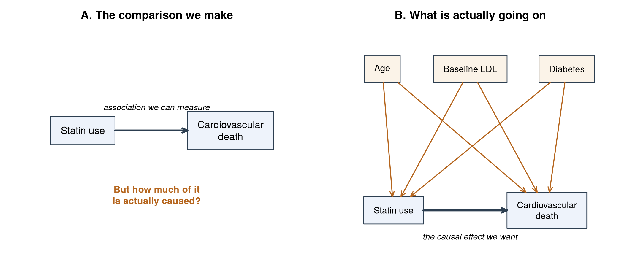
Figure 22.1 makes the point with a familiar example: statins and cardiovascular death.
Panel B is the honest picture, and it explains why the naive comparison misleads. Older patients are more likely to be prescribed a statin and more likely to die of cardiovascular disease. So are patients with high baseline LDL, and patients with diabetes. Each of those three variables therefore supplies a route from “statin use” to “cardiovascular death” that has nothing to do with the drug doing anything. Any observed association is a mixture of the real effect (thick arrow) and those three spurious routes.
That is the whole job of the rest of this chapter: close the gold routes, keep the thick one.
22.3.2 The three structures you must recognise
Not every variable in a DAG should be adjusted for. This is the single most consequential thing to get right, and it comes down to recognising three shapes (Figure 22.2). Two of them look superficially similar and demand opposite treatment.
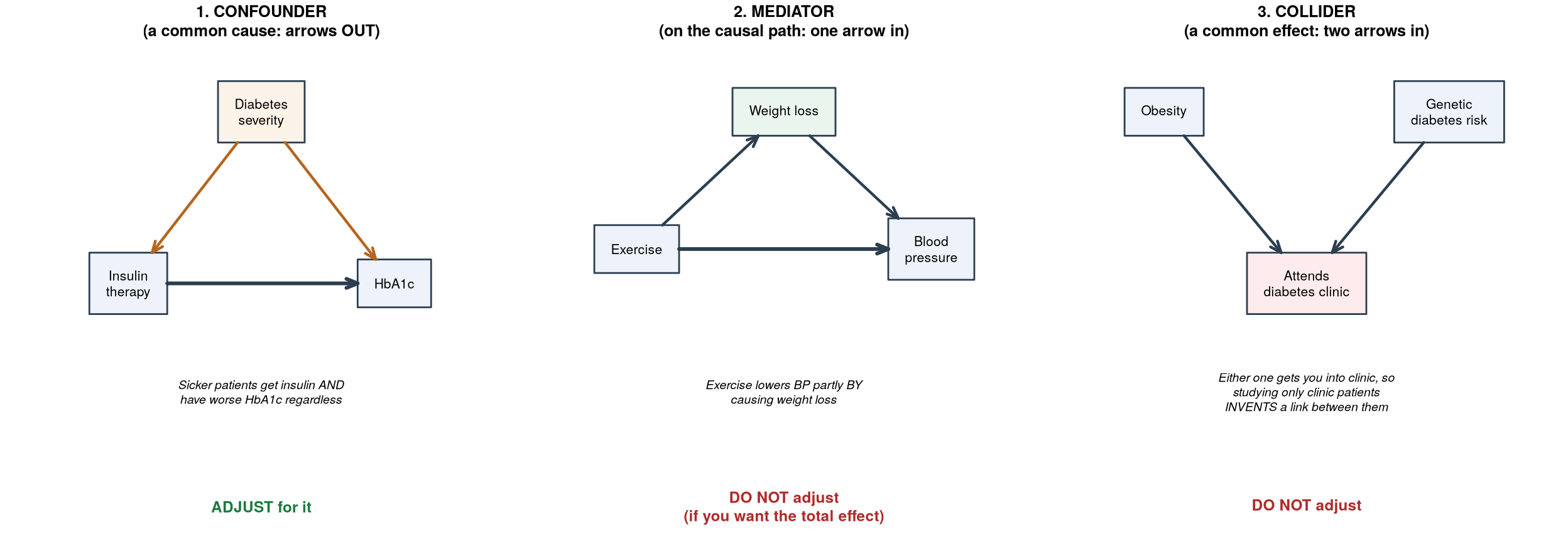
1. Confounders (common causes) — adjust. A variable with an arrow into both the treatment and the outcome. In the first panel of Figure 22.2, diabetes severity is a common cause of insulin therapy and of HbA1c: sicker patients are more likely to be started on insulin, and they tend to have a higher HbA1c whatever the insulin does. Leave diabetes severity out of the analysis and insulin will look useless, or even harmful.
2. Mediators (intermediate variables) — do not adjust, if you want the total effect. A variable on the causal pathway from treatment to outcome. In the middle panel, exercise lowers blood pressure partly by causing weight loss, so part of exercise’s benefit is the weight loss. Adjusting for weight loss asks “what does exercise do for patients whose weight did not change?”, which is a different (and usually not the intended) question. Decomposing an effect into its mediated and unmediated parts on purpose is the subject of Chapter 23.
3. Colliders (common effects) — do not adjust. A collider is a variable that is caused by both the treatment and the outcome (or by variables on each path) — the two arrows “collide” into it. This is the counter-intuitive case: adjusting for a collider creates an association that was not there.
Why does that happen? Take the clinic example. Suppose obesity and genetic diabetes risk are entirely unrelated in the general population, but either one is enough to get you referred to a diabetes clinic. Now look only at clinic attendees. If you meet a slim patient in the clinic, you can infer they are probably there for the genetic risk — because something got them referred, and it was not their weight. So among clinic patients, being slim now predicts high genetic risk. The association is real within the clinic and completely absent outside it. You manufactured it by looking only at the clinic. That is collider bias, and its commonest disguise in clinical research is a study restricted to hospitalised patients, or one that adjusts for a post-treatment variable such as “was admitted to ICU”.
TipThe “d-separation” rule of thumb
A path between treatment and outcome is blocked if:
- It passes through a variable you condition on (confounder or mediator), OR
- It passes through a collider you do NOT condition on.
A path is open if it is not blocked. Bias creeps in when there are open non-causal paths between treatment and outcome — so-called backdoor paths, sneaky side-routes (usually running through a confounder) that make treatment and outcome look related even when the treatment does nothing. The goal of adjustment is to close every backdoor path while leaving the genuine causal path alone.
22.3.3 A full clinical DAG, and what to do with it
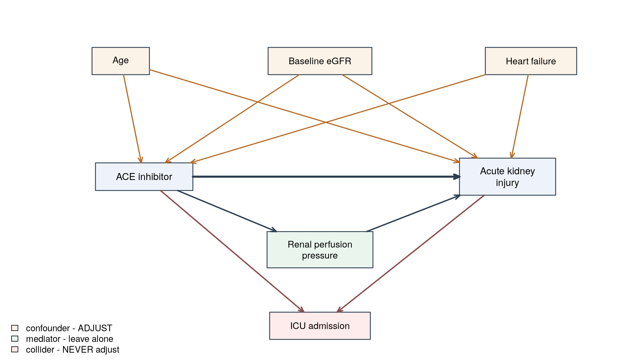
Real DAGs contain all three shapes at once. Figure 22.3 is a realistic (if simplified) diagram for a question you might genuinely be asked: do ACE inhibitors cause acute kidney injury in hospitalised patients?
Reading it off:
- Age, baseline eGFR, and heart failure are confounders. Each is a reason a clinician prescribes an ACE inhibitor and an independent risk factor for AKI. All three must be adjusted for.
- Renal perfusion pressure is a mediator. Part of how ACE inhibitors precipitate AKI is by reducing perfusion pressure. If you want the drug’s total effect on AKI, leave it out. Put it in and you will conclude the drug is safer than it is.
- ICU admission is a collider. Patients go to ICU because of ACEi-related complications and because of AKI. Adjust for it — or, just as damagingly, run the whole study in an ICU cohort — and you will find an association whatever the truth.
You do not have to trace the paths by hand. The dagitty package (the R interface to the DAGitty web tool) does it for you, and the point of writing the DAG down in code is that the adjustment set is then derived rather than guessed:
Code
# install.packages("dagitty")
library(dagitty)   # encode a DAG and derive adjustment sets from it

# NOTE: dagitty's DAG syntax is NOT R. In particular it has no comments ---
# a `#` inside the dag{...} string is a syntax error. Keep explanations
# outside the quotes, as ordinary R comments like this one.
aki_dag <- dagitty('dag {
  ACEi          [exposure]
  AKI           [outcome]

  Age           -> ACEi
  Age           -> AKI
  BaselineEGFR  -> ACEi
  BaselineEGFR  -> AKI
  HeartFailure  -> ACEi
  HeartFailure  -> AKI

  ACEi          -> AKI
  ACEi          -> RenalPerfusion
  RenalPerfusion -> AKI

  ACEi          -> ICUAdmission
  AKI           -> ICUAdmission
}')

# What must we adjust for to get the TOTAL effect of ACEi on AKI?
adjustmentSets(aki_dag, type = "minimal", effect = "total")

# Which variables are colliders we must leave alone? Ask dagitty what
# happens to the estimate if we wrongly condition on ICU admission:
adjustmentSets(aki_dag, type = "minimal", effect = "total") # {Age, BaselineEGFR, HeartFailure}
impliedConditionalIndependencies(aki_dag)
What the code shows. dagitty() turns the picture into an object; adjustmentSets() then applies the backdoor criterion and returns the minimal set of variables that closes every backdoor path — here {Age, BaselineEGFR, HeartFailure}. Note what it does not include: RenalPerfusion (a mediator) and ICUAdmission (a collider). Getting that list from an algorithm rather than from intuition is the entire reason to draw the DAG in the first place. impliedConditionalIndependencies() goes further and lists the independence relations your DAG predicts, several of which you can actually go and test in your data — a rare opportunity to check a causal assumption empirically.
22.3.4 Drawing your own DAG
Before any causal analysis, draw a DAG. Steps:
- List all variables relevant to treatment assignment and the outcome.
- Use clinical knowledge to draw arrows (not data — DAGs encode assumptions).
- Identify all backdoor paths from treatment to outcome.
- Determine the minimal adjustment set that blocks all backdoor paths without opening new ones.
Tools like DAGitty automate steps 3 and 4 once you have drawn the DAG, either in the browser or from R via dagitty as above.
22.4 Propensity Score Methods
22.4.1 The propensity score
The propensity score is each patient’s probability of receiving the treatment, based on their observed characteristics. Think of it as: “given everything I know about this patient, how likely was a clinician to put them on this drug?”
\[ \underbrace{e(L)}_{\text{propensity score}} = \underbrace{P(A = 1 \mid L)}_{\substack{\text{chance of being treated, for a patient}\\ \text{with these characteristics } L}} \]
Rosenbaum and Rubin (1983) showed something remarkably useful: if exchangeability holds once we account for all the covariates \(L\), then it also holds once we account for just this single number \(e(L)\). So instead of trying to balance dozens of patient characteristics one by one, we only need to balance one summary score. That is why propensity scores are so popular in clinical research — they turn an unwieldy problem into a manageable one.
22.4.2 The running example
Every code block from here on uses the same simulated cohort, so that the different methods can be compared on identical data. Each chunk re-creates the cohort in full, so any chunk can be copied and run on its own.
The set-up is confounding by indication, deliberately built in:
- 4000 patients described by age, eGFR (kidney function), and whether they have a major comorbidity;
- older patients, patients with worse kidney function, and patients with a comorbidity are more likely to be treated — this is the clinician acting on illness severity;
- those same three characteristics also raise the risk of death, independently of treatment;
- and the drug genuinely works: we hard-wire a protective effect (a log-odds of \(-0.8\)).
Because we built the data, we know the right answer. Averaged over this cohort’s mix of patients, the true effect on the risk scale is a risk difference of \(-0.130\): treating everyone rather than nobody would prevent 13 deaths per 100 patients. Any method worth using should get close to that. The naive comparison, as we will see, gets nowhere near it.
22.4.3 Estimating the propensity score
We typically estimate \(e(L)\) using logistic regression (or more flexible methods like gradient boosting):
Code
library(tidyverse)   # tibble(), mutate(), ggplot2

# --- The running cohort: confounding by indication, known true effect --------
set.seed(42)
n <- 4000

dat <- tibble(
  age      = rnorm(n, 65, 10),
  egfr     = rnorm(n, 60, 15),
  comorbid = rbinom(n, 1, 0.4)
) |>
  mutate(
    # Sicker patients (older, worse kidneys, comorbid) are MORE likely treated
    treat = rbinom(n, 1, plogis(-0.8 + 0.05 * (age - 65) -
                                  0.04 * (egfr - 60) + 0.8 * comorbid)),
    # Those same characteristics also raise mortality; the drug is protective
    death = rbinom(n, 1, plogis(-1.2 + 0.05 * (age - 65) -
                                  0.035 * (egfr - 60) + 0.7 * comorbid -
                                  0.8 * treat))
  )

# --- Estimate the propensity score: P(treated | characteristics) -------------
ps_model <- glm(treat ~ age + egfr + comorbid, data = dat, family = binomial)
dat$ps <- predict(ps_model, type = "response")

# --- Check OVERLAP: do the two groups occupy the same range of scores? -------
ggplot(dat, aes(x = ps, fill = factor(treat, labels = c("Untreated", "Treated")))) +
  geom_density(alpha = 0.5) +
  labs(
    x = "Propensity score (estimated probability of being treated)",
    y = "Density", fill = NULL,
    title = "Propensity score distribution by treatment group"
  ) +
  theme_minimal()
Code
import numpy as np
import pandas as pd
import matplotlib.pyplot as plt
import statsmodels.formula.api as smf

# --- The running cohort: confounding by indication, known true effect --------
rng = np.random.default_rng(42)
n = 4000

age      = rng.normal(65, 10, n)
egfr     = rng.normal(60, 15, n)
comorbid = rng.binomial(1, 0.4, n)

expit = lambda x: 1 / (1 + np.exp(-x))

treat = rng.binomial(1, expit(-0.8 + 0.05*(age-65) - 0.04*(egfr-60) + 0.8*comorbid))
death = rng.binomial(1, expit(-1.2 + 0.05*(age-65) - 0.035*(egfr-60)
                              + 0.7*comorbid - 0.8*treat))

df = pd.DataFrame(dict(age=age, egfr=egfr, comorbid=comorbid,
                       treat=treat, death=death))

# --- Estimate the propensity score: P(treated | characteristics) -------------
ps_model = smf.logit("treat ~ age + egfr + comorbid", data=df).fit(disp=0)
df["ps"] = ps_model.predict(df)

# --- Check OVERLAP: do the two groups occupy the same range of scores? -------
fig, ax = plt.subplots(figsize=(8, 4.5))
for value, label in [(0, "Untreated"), (1, "Treated")]:
    df.loc[df.treat == value, "ps"].plot.density(ax=ax, alpha=0.6, label=label)
ax.set_xlabel("Propensity score (estimated probability of being treated)")
ax.set_ylabel("Density")
ax.set_title("Propensity score distribution by treatment group")
ax.legend()
plt.tight_layout()
plt.show()
What the code shows. We simulate the running cohort described above, then fit a logistic regression of treatment on the three characteristics; its fitted probabilities are the propensity scores. The density plot shows those scores separately for treated and untreated patients. What you want to see is substantial overlap between the two curves: that means for most patients there exist comparable patients in the other group. If the two curves barely overlap — treated patients piled up near 1, controls near 0 — the groups are too different to compare fairly, which is the warning below.
WarningPositivity assumption
Positivity means every type of patient must have at least some chance of receiving either treatment — nobody is guaranteed to be treated or guaranteed to be untreated. If a group of patients always gets the drug (propensity score near 1) or never gets it (near 0), there are no comparable patients in the other arm, so the comparison breaks down and estimates become unstable. Always check the propensity score distributions visually.
22.4.4 Propensity score matching
Matching pairs each treated patient with one (or more) untreated patient who had a similar propensity score — in effect, finding each treated patient a “statistical twin” who looked equally likely to be treated but happened not to be. Comparing these matched pairs mimics what a randomised trial does naturally: it puts like next to like.
Code
library(tidyverse)  # tibble(), mutate()
library(MatchIt)    # matchit(), match.data()
library(cobalt)     # love.plot(), bal.tab()
library(broom)      # tidy() -- WITHOUT this, tidy() on a glm fails

# --- The running cohort (see above; repeated so this chunk stands alone) -----
set.seed(42)
n <- 4000
dat <- tibble(
  age      = rnorm(n, 65, 10),
  egfr     = rnorm(n, 60, 15),
  comorbid = rbinom(n, 1, 0.4)
) |>
  mutate(
    treat = rbinom(n, 1, plogis(-0.8 + 0.05 * (age - 65) -
                                  0.04 * (egfr - 60) + 0.8 * comorbid)),
    death = rbinom(n, 1, plogis(-1.2 + 0.05 * (age - 65) -
                                  0.035 * (egfr - 60) + 0.7 * comorbid -
                                  0.8 * treat))
  )

# --- 1:1 nearest-neighbour matching on the propensity score -----------------
m_out <- matchit(treat ~ age + egfr + comorbid,
  data = dat,
  method = "nearest",
  distance = "glm",   # propensity score from logistic regression
  caliper = 0.2,      # refuse matches further apart than 0.2 SD of logit(PS)
  ratio = 1           # one control per treated patient
)

m_out                      # how many patients matched, how many dropped
bal.tab(m_out, thresholds = c(m = 0.1))   # balance table, numerically

# --- Did matching work? The Love plot is the standard visual check ----------
love.plot(m_out,
  thresholds = c(m = 0.1),
  binary = "std",
  title = "Covariate balance: before and after matching"
)

# --- Estimate the effect in the matched sample ------------------------------
m_data <- match.data(m_out)

outcome_model <- glm(death ~ treat,
  data = m_data,
  family = binomial,
  weights = weights   # match.data() supplies these
)

tidy(outcome_model, conf.int = TRUE, exponentiate = TRUE)
ImportantThe two mistakes that make this chunk fail
Both are easy to hit if you copy code out of a paper rather than out of a script that was actually run.
library(MatchIt)andlibrary(cobalt)must be loaded. Without them,matchit()andlove.plot()do not exist. The error message (could not find function "matchit") is at least clear.library(broom)must be loaded fortidy(). This one is nastier, because several modelling packages re-export the generictidy()without providing the methods for it. Sotidy()is found, but has no idea what to do with aglm, and you get the baffling:Error in UseMethod("tidy") : no applicable method for 'tidy' applied to an object of class "c('glm', 'lm')"That message reads like a problem with your model. It is not — it means
broomis missing. Load it and the same line works.
What the code shows. matchit() pairs each treated patient with the most similar untreated patient by propensity score, refusing any match further apart than the caliper (0.2 standard deviations of the logit score). Printing m_out reports how many patients were matched — and, importantly, how many were dropped: in this cohort 1380 of the 1582 treated patients find a partner and 202 do not, which changes the population your estimate refers to. bal.tab() gives the numbers and love.plot() draws the picture: one dot per covariate showing the standardised mean difference (SMD) before matching and after. The SMD is just the difference in a covariate’s mean between treated and control groups, divided by its standard deviation — a unit-free measure of how far apart the groups are. The whole point of matching is to pull every “after” dot inside the 0.1 reference line. Finally we estimate the treatment effect on the matched sample; with exponentiate = TRUE the treat row is an odds ratio for death (about 0.51 here, so a substantial protective effect), with its 95% confidence interval.
Checking balance is the most important step after matching. An SMD below 0.1 for all covariates is the conventional threshold for acceptable balance. Balance, here, simply means the treated and control groups have a similar mix of patients — the situation a randomised trial would create automatically, and what we are trying to recreate by hand.
NoteMatching gives you the ATT, and throws patients away
Two consequences of matching that catch people out. First, because we matched to the treated patients, the estimate is the ATT — the effect among patients like those who were actually treated — not the ATE. Second, unmatched patients are simply discarded. That is a real loss of information, and if the discarded patients are systematically different (they usually are: they are the most extreme ones), the population your answer applies to has quietly shifted. The next section avoids both problems.
22.5 Estimating the Effect: Weighting and G-Computation
Matching balances the groups by throwing patients away. There are two better-behaved workhorses that use the whole sample, and both come from the work of the epidemiologist James Robins, who called them the g-methods (“g” for generalised):
- Inverse probability weighting (IPW) models who gets treated. It builds a re-weighted “pseudo-population” in which treatment is no longer tied to the confounders, then compares outcomes in that pseudo-population.
- G-computation (also called the parametric g-formula, or standardisation) models what the outcome would be. It fits an outcome model, then uses it to predict every patient’s outcome twice — once as if treated, once as if untreated — and contrasts the averages.
Both target the ATE, and under the same core assumption (no unmeasured confounding) both recover it. It is worth knowing both, because they place their bets on different models, and agreement between them is itself reassuring.
ImportantWhy not just read the coefficient off a regression?
A naive analyst fits death ~ treat + age + egfr + comorbid and reads off the treat coefficient. The trouble is that a regression coefficient is only the causal effect under restrictive conditions: no treatment-covariate interactions, correct functional form, and a collapsible effect measure (which the odds ratio is not). The g-methods sidestep these traps by computing the effect the way its definition demands — as a contrast of average potential outcomes — rather than trusting one coefficient to mean what we hope it means.
22.5.1 Inverse probability weighting
The idea in plain language
Instead of discarding anyone, IPW keeps the whole sample but gives each patient a weight, so that after weighting the treated and untreated groups have the same mix of characteristics.
Here is the intuition, set out accessibly for clinical readers by Mansournia and Altman (2016) and Chesnaye et al. (2022). Suppose a very sick patient — the kind clinicians almost always treat — nevertheless went untreated. That patient is rare and precious: they are one of the few untreated people who look like the treated group, so they carry a lot of information about what happens to treated-type patients when they go without the drug. IPW gives such a patient a large weight. Conversely, an untreated patient who looked very unlikely to be treated anyway is over-represented among controls, so IPW shrinks their weight. Do this for everyone and you build a pseudo-population in which being treated is statistically unrelated to the confounders — exactly the situation a randomised trial creates by design.
The weight for each patient is the inverse of the probability of the treatment they actually received:
\[ w_i = \underbrace{\frac{A_i}{e(L_i)}}_{\substack{\text{for treated patients:}\\ 1 \,/\, \text{chance of being treated}}} + \underbrace{\frac{1 - A_i}{1 - e(L_i)}}_{\substack{\text{for untreated patients:}\\ 1 \,/\, \text{chance of being untreated}}} \]
A treated patient with propensity score 0.2 gets weight \(1/0.2 = 5\); an untreated patient with propensity score 0.9 (so a probability of being untreated of 0.1) gets weight \(1/0.1 = 10\). These weights are larger precisely for the informative, “surprising” patients. This version estimates the ATE. For the ATT, the weights instead are \(w_i = A_i + (1 - A_i)\,e(L_i) / (1 - e(L_i))\): treated patients keep weight 1, and controls are re-weighted to look like them.
Stabilised weights
The raw weights can occasionally become enormous — if a treated patient had a propensity score of 0.01, their weight is 100, and a single patient can then dominate the analysis and inflate the variance. Stabilised weights tame this by replacing the “1” in the numerator with the overall probability of receiving that treatment:
\[ sw_i = \frac{A_i \cdot P(A = 1)}{e(L_i)} + \frac{(1 - A_i) \cdot P(A = 0)}{1 - e(L_i)} \]
The estimate is unchanged on average, but the weights cluster sensibly around 1 and the confidence intervals are narrower and more honest. Stabilised weights are the default recommendation and what modern packages produce automatically.
NoteMarginal structural models in one line
When you fit an outcome model (say, a regression of mortality on treatment) using these weights, the model you have fitted is called a marginal structural model (MSM). “Marginal” because it describes the whole population (not conditional on confounders), and “structural” because its coefficients have a causal interpretation. MSMs are the natural home of IPW and the standard tool when a treatment changes over time — a setting where ordinary regression genuinely cannot give the right answer.
Two checks that are not optional
Weighting is only trustworthy if it actually balanced the confounders, and only valid if every kind of patient could in principle have received either treatment:
- Covariate balance. After weighting, the treated and control groups should have a near-identical mix of confounders. Measure this with the standardised mean difference and want every value comfortably below 0.1.
- Positivity. A propensity score near 0 or 1 produces an explosive weight. Inspect the largest weights: a maximum above roughly 10–20 is a warning that positivity is shaky and the estimate may be unstable.
IPW in practice
Code
library(tidyverse)       # tibble(), mutate()
library(WeightIt)        # weightit(), glm_weightit() -- MUST be loaded
library(cobalt)          # bal.tab() -- MUST be loaded
library(marginaleffects) # avg_comparisons()

# --- The running cohort (repeated so this chunk stands alone) ---------------
set.seed(42)
n <- 4000
dat <- tibble(
  age      = rnorm(n, 65, 10),
  egfr     = rnorm(n, 60, 15),
  comorbid = rbinom(n, 1, 0.4)
) |>
  mutate(
    treat = rbinom(n, 1, plogis(-0.8 + 0.05 * (age - 65) -
                                  0.04 * (egfr - 60) + 0.8 * comorbid)),
    death = rbinom(n, 1, plogis(-1.2 + 0.05 * (age - 65) -
                                  0.035 * (egfr - 60) + 0.7 * comorbid -
                                  0.8 * treat))
  )

# --- Step 1: stabilised weights for the ATE --------------------------------
W <- weightit(treat ~ age + egfr + comorbid,
  data = dat, method = "glm", estimand = "ATE", stabilize = TRUE
)

# --- Step 2: the two mandatory checks --------------------------------------
bal.tab(W, thresholds = c(m = 0.1))   # balance: want every SMD < 0.1
summary(W)                            # positivity: inspect the largest weights

# --- Step 3: the weighted outcome model (a marginal structural model) ------
msm <- glm_weightit(death ~ treat, data = dat, weightit = W, family = binomial)

# --- Step 4: convert it to a risk difference ------------------------------
#   variables = list(treat = 0:1) makes the 0 -> 1 contrast explicit
avg_comparisons(msm, variables = list(treat = 0:1))
What the code shows. weightit() estimates the propensity score and converts it into stabilised ATE weights in one call. bal.tab() prints a table of standardised mean differences for age, egfr, and comorbid after weighting — every number here comes out under 0.03, comfortably inside the 0.1 threshold, confirming the pseudo-population is balanced. summary(W) reports the range of weights; the maximum here is about 6, well under 20, so positivity is not violated. It also prints the effective sample size, which falls from 4000 to about 3300 — that drop is the price of the re-weighting, and it is why the confidence interval is a little wider than an unweighted one would be. Finally glm_weightit() fits the weighted outcome model — this is the marginal structural model — and avg_comparisons() converts it into a risk difference: the average change in the probability of death caused by the drug, with a confidence interval that correctly accounts for the weighting. You should get about \(-0.124\) (95% CI \(-0.150\) to \(-0.097\)), which brackets the true \(-0.130\).
TipWhy
glm_weightit() and not glm(..., weights = )?
Plain glm() will accept the weights and give you the right point estimate, but the standard error will be wrong — it treats the weights as if they were known counts of real patients, when in fact they were estimated from the propensity model. glm_weightit() (or a survey-design fit via survey::svyglm()) accounts for that estimation step and gives an honest, slightly wider interval. If you use svyglm(), remember library(broom) before tidy(), for exactly the reason flagged in the matching section.
Code
import numpy as np
import pandas as pd
import statsmodels.api as sm
import statsmodels.formula.api as smf

# --- The running cohort (repeated so this chunk stands alone) ---------------
rng = np.random.default_rng(42)
n = 4000
expit = lambda x: 1 / (1 + np.exp(-x))

age      = rng.normal(65, 10, n)
egfr     = rng.normal(60, 15, n)
comorbid = rng.binomial(1, 0.4, n)
treat = rng.binomial(1, expit(-0.8 + 0.05*(age-65) - 0.04*(egfr-60) + 0.8*comorbid))
death = rng.binomial(1, expit(-1.2 + 0.05*(age-65) - 0.035*(egfr-60)
                              + 0.7*comorbid - 0.8*treat))
df = pd.DataFrame(dict(age=age, egfr=egfr, comorbid=comorbid,
                       treat=treat, death=death))

# --- Step 1: propensity score, then stabilised weights ---------------------
df["ps"] = smf.logit("treat ~ age + egfr + comorbid", data=df).fit(disp=0).predict(df)

p_treat = df["treat"].mean()
df["sw"] = np.where(df["treat"] == 1,
                    p_treat / df["ps"],
                    (1 - p_treat) / (1 - df["ps"]))

# --- Step 2: the two mandatory checks -------------------------------------
def weighted_smd(var):
    t, c = df[df.treat == 1], df[df.treat == 0]
    mt = np.average(t[var], weights=t.sw)
    mc = np.average(c[var], weights=c.sw)
    sd = np.sqrt((t[var].var() + c[var].var()) / 2)
    return (mt - mc) / sd

print("Balance after weighting (want |SMD| < 0.1):")
for v in ["age", "egfr", "comorbid"]:
    print(f"  {v:<9} {weighted_smd(v):+.3f}")
print(f"Positivity check -- largest weight: {df['sw'].max():.2f}")

# --- Steps 3 and 4: weighted outcome model -> risk difference -------------
msm = smf.glm("death ~ treat", data=df, family=sm.families.Binomial(),
              freq_weights=df["sw"]).fit()

rd = (msm.predict(df.assign(treat=1)) - msm.predict(df.assign(treat=0))).mean()
print(f"\nIPW risk difference (treated - untreated): {rd:+.4f}")
What the code shows. The same workflow written out step by step, so nothing is hidden. We fit a logistic propensity-score model, build stabilised weights by hand from the formula above, and then run the two checks: the weighted standardised mean differences should all sit near zero, and the largest weight should be nowhere near 20. We then fit the weighted outcome model and, rather than reading a single coefficient, predict every patient’s death probability twice (everyone treated, then everyone untreated) and average the difference. That average is the risk difference, directly comparable to the R output, and it should be close to the true \(-0.130\).
Two caveats specific to this hand-rolled version. First, statsmodels will report a standard error that ignores the fact that the weights were estimated, so it is somewhat too narrow; bootstrap the whole procedure if you need an honest interval. Second, freq_weights expects the weights to behave like counts — fine for the point estimate, another reason not to trust the printed standard error.
22.5.2 G-computation
The idea in plain language
IPW models the treatment. G-computation instead models the outcome, and it follows the definition of the ATE almost literally.
Recall the definition: the average outcome if everyone were treated minus the average outcome if everyone were untreated. We never observe both worlds for any patient — but we can predict them. The recipe has three steps:
- Fit one outcome model that includes treatment and all the confounders (and, ideally, their interactions). This model learns how the outcome depends jointly on treatment and patient characteristics.
- Predict twice for every patient. First set everyone’s treatment to “treated” (leaving their real confounders untouched) and predict each patient’s outcome. Then reset everyone to “untreated” and predict again. Each patient now has two predicted outcomes — their estimated potential outcomes.
- Average and contrast. Average the “all treated” predictions, average the “all untreated” predictions, and take the difference. That difference is the average treatment effect.
This procedure is also called standardisation, because it standardises both arms to the same confounder distribution (the whole sample’s). It is the oldest idea in the chapter — Robins introduced the g-formula in 1986 — and it remains one of the most reliable.
graph LR
    A["Fit outcome model:<br/>outcome ~ treatment<br/>+ confounders"] --> B["Predict each patient<br/>as if TREATED"]
    A --> C["Predict each patient<br/>as if UNTREATED"]
    B --> D["Average each set,<br/>then subtract"]
    C --> D
    D --> E["Average treatment<br/>effect"]
    style A fill:#eef3fb,color:#111
    style B fill:#eef3fb,color:#111
    style C fill:#eef3fb,color:#111
    style D fill:#eef3fb,color:#111
    style E fill:#eef3fb,color:#111
Confidence intervals: use the bootstrap
Because g-computation predicts, averages, and contrasts, the uncertainty in the final number does not come out of the outcome model directly. The standard solution is the bootstrap: resample the patients with replacement many times, rerun the whole predict-average-contrast procedure on each resample, and use the spread of the resulting estimates as the confidence interval. In R, marginaleffects::inferences() wraps the bootstrap around the whole calculation.
G-computation in practice
Code
library(tidyverse)       # tibble(), mutate()
library(marginaleffects) # avg_comparisons(), inferences()

# --- The running cohort (repeated so this chunk stands alone) ---------------
set.seed(42)
n <- 4000
dat <- tibble(
  age      = rnorm(n, 65, 10),
  egfr     = rnorm(n, 60, 15),
  comorbid = rbinom(n, 1, 0.4)
) |>
  mutate(
    treat = rbinom(n, 1, plogis(-0.8 + 0.05 * (age - 65) -
                                  0.04 * (egfr - 60) + 0.8 * comorbid)),
    death = rbinom(n, 1, plogis(-1.2 + 0.05 * (age - 65) -
                                  0.035 * (egfr - 60) + 0.7 * comorbid -
                                  0.8 * treat))
  )

# --- Step 1: ONE outcome model, with treatment-confounder interactions -----
#   The interactions let the drug's effect differ across patient types.
out_model <- glm(death ~ treat * (age + egfr + comorbid),
  data = dat, family = binomial
)

# --- Steps 2 and 3: predict under treat = 1 and treat = 0, average, contrast
#   avg_comparisons() does the standardisation; inferences() bootstraps the CI
avg_comparisons(out_model, variables = list(treat = 0:1)) |>
  inferences(method = "boot", R = 500)

# --- The same thing by hand, to show there is no magic --------------------
p1 <- predict(out_model, transform(dat, treat = 1), type = "response")
p0 <- predict(out_model, transform(dat, treat = 0), type = "response")
mean(p1) - mean(p0)
What the code shows. We fit a single logistic outcome model, deliberately including treat * (age + egfr + comorbid) so the drug’s effect is allowed to differ across patient types — flexibility that a plain regression coefficient cannot express. avg_comparisons(..., variables = list(treat = 0:1)) carries out the g-computation: it predicts every patient’s death probability with treat set to 1, again with it set to 0, averages each, and reports the difference as a risk difference. Piping into inferences(method = "boot", R = 500) wraps the whole procedure in a 500-replicate bootstrap so the confidence interval is honest. The estimate comes out near \(-0.122\) — close to the true \(-0.130\) and to the IPW estimate. The last two lines do the same calculation manually and print the identical number, which is worth running once so that the function stops feeling like a black box.
Code
import numpy as np
import pandas as pd
import statsmodels.api as sm
import statsmodels.formula.api as smf

# --- The running cohort (repeated so this chunk stands alone) ---------------
rng = np.random.default_rng(42)
n = 4000
expit = lambda x: 1 / (1 + np.exp(-x))

age      = rng.normal(65, 10, n)
egfr     = rng.normal(60, 15, n)
comorbid = rng.binomial(1, 0.4, n)
treat = rng.binomial(1, expit(-0.8 + 0.05*(age-65) - 0.04*(egfr-60) + 0.8*comorbid))
death = rng.binomial(1, expit(-1.2 + 0.05*(age-65) - 0.035*(egfr-60)
                              + 0.7*comorbid - 0.8*treat))
df = pd.DataFrame(dict(age=age, egfr=egfr, comorbid=comorbid,
                       treat=treat, death=death))

# --- The g-computation procedure, as a reusable function ------------------
def gcomp(data):
    m = smf.glm("death ~ treat * (age + egfr + comorbid)",
                data=data, family=sm.families.Binomial()).fit(disp=0)
    return (m.predict(data.assign(treat=1)).mean()
            - m.predict(data.assign(treat=0)).mean())

point = gcomp(df)

# --- Bootstrap the confidence interval ----------------------------------
boot_rng = np.random.default_rng(1)
boot = np.array([
    gcomp(df.iloc[boot_rng.integers(0, len(df), len(df))])
    for _ in range(500)
])
lo, hi = np.percentile(boot, [2.5, 97.5])
print(f"G-computation risk difference: {point:+.4f} (95% CI {lo:+.4f}, {hi:+.4f})")
What the code shows. We wrap the predict-average-contrast recipe in a function, gcomp(), that fits the interaction outcome model, predicts every patient’s death probability under “everyone treated” and “everyone untreated”, and returns the average difference. Calling it once on the real data gives the point estimate. We then call it 500 more times on bootstrap resamples (patients drawn with replacement) and take the 2.5th and 97.5th percentiles as a 95% confidence interval. The printed risk difference should be close to the true \(-0.130\), and to the R result.
TipA ready-made alternative in R
You do not have to hand-roll the outcome model. The stdReg2 package implements standardisation (g-computation) directly with built-in confidence intervals, and for time-varying treatments — where a patient’s treatment and confounders evolve over follow-up, and ordinary methods break down — the gfoRmula package implements the full longitudinal parametric g-formula. We use the glm + marginaleffects route here because it makes every step transparent, but stdReg2 is an excellent production tool.
22.5.3 Putting it together: naive vs IPW vs g-computation
The point of all this is best seen in one picture. Figure 22.5 estimates the drug’s effect three ways on identical data: a naive regression that ignores confounding, IPW, and g-computation — against the true answer, which we know because we built it.
Code
library(tidyverse)       # tibble(), bind_rows(), ggplot2
library(WeightIt)        # weightit(), glm_weightit()
library(marginaleffects) # avg_comparisons()

# --- The running cohort -----------------------------------------------------
set.seed(42)
n <- 4000
dat <- tibble(
  age      = rnorm(n, 65, 10),
  egfr     = rnorm(n, 60, 15),
  comorbid = rbinom(n, 1, 0.4)
) |>
  mutate(
    treat = rbinom(n, 1, plogis(-0.8 + 0.05 * (age - 65) -
                                  0.04 * (egfr - 60) + 0.8 * comorbid)),
    death = rbinom(n, 1, plogis(-1.2 + 0.05 * (age - 65) -
                                  0.035 * (egfr - 60) + 0.7 * comorbid -
                                  0.8 * treat))
  )

# The truth, computable only because we wrote the data-generating model
TRUE_RD <- -0.130

# (a) NAIVE: ignore the confounders entirely
naive_rd <- avg_comparisons(
  glm(death ~ treat, data = dat, family = binomial),
  variables = list(treat = 0:1)
)

# (b) IPW: stabilised weights + weighted outcome model
W <- weightit(treat ~ age + egfr + comorbid, data = dat,
              method = "glm", estimand = "ATE", stabilize = TRUE)
ipw_rd <- avg_comparisons(
  glm_weightit(death ~ treat, data = dat, weightit = W, family = binomial),
  variables = list(treat = 0:1)
)

# (c) G-COMPUTATION: outcome model + standardisation
gcomp_rd <- avg_comparisons(
  glm(death ~ treat * (age + egfr + comorbid), data = dat, family = binomial),
  variables = list(treat = 0:1)
)

results <- bind_rows(
  tibble(method = "Naive regression\n(ignores confounders)", as_tibble(naive_rd)),
  tibble(method = "IPW\n(models treatment)", as_tibble(ipw_rd)),
  tibble(method = "G-computation\n(models outcome)", as_tibble(gcomp_rd))
) |>
  select(method, estimate, conf.low, conf.high) |>
  mutate(method = factor(method, levels = rev(method)))

print(as.data.frame(results), digits = 3)

ggplot(results, aes(x = estimate, y = method)) +
  geom_vline(xintercept = 0, colour = "grey55") +
  geom_vline(xintercept = TRUE_RD, colour = "#b02a2a",
             linetype = "dashed", linewidth = 0.8) +
  geom_errorbar(aes(xmin = conf.low, xmax = conf.high),
                width = 0.16, linewidth = 0.8, colour = "#2c3e50") +
  geom_point(size = 3.6, colour = "#2c3e50") +
  annotate("text", x = TRUE_RD, y = 3.45, hjust = 0, size = 3.6,
           fontface = "bold", colour = "#b02a2a",
           label = "  TRUE effect (-0.130)") +
  annotate("text", x = 0, y = 3.45, hjust = 1.05, size = 3.4,
           colour = "grey40", label = "no effect  ") +
  scale_x_continuous(limits = c(-0.20, 0.035)) +
  labs(x = "Risk difference in mortality (treated - untreated)", y = NULL) +
  theme_minimal(base_size = 12) +
  theme(panel.grid.major.y = element_blank(),
        plot.margin = margin(16, 14, 6, 6))
method estimate conf.low conf.high
1 Naive regression\n(ignores confounders) -0.0322 -0.0592 -0.00517
2 IPW\n(models treatment) -0.1236 -0.1504 -0.09669
3 G-computation\n(models outcome) -0.1219 -0.1478 -0.09592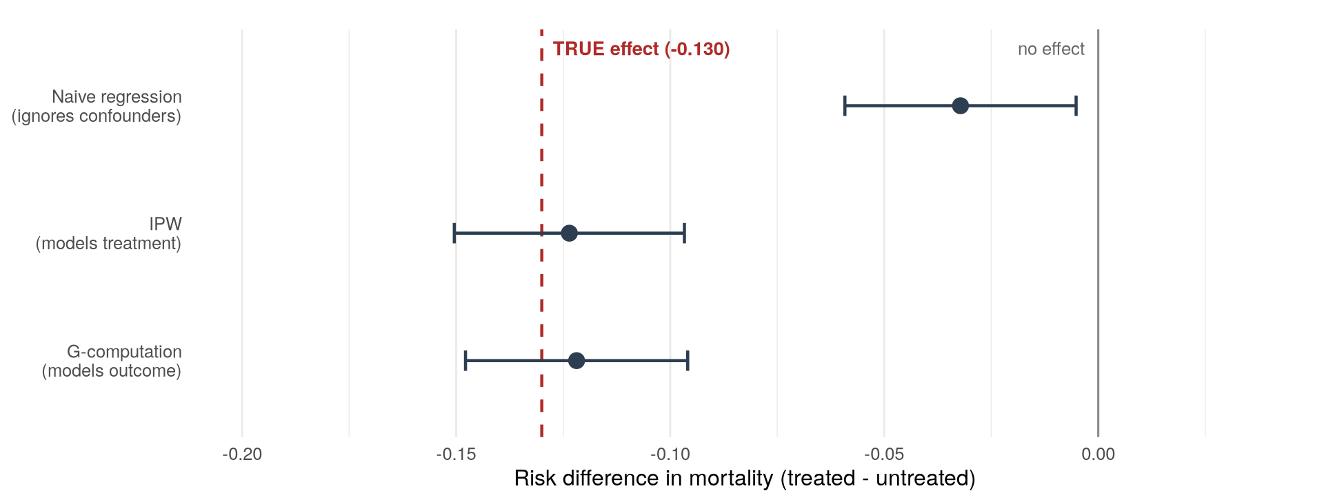
Code
import numpy as np
import pandas as pd
import matplotlib.pyplot as plt
import statsmodels.api as sm
import statsmodels.formula.api as smf

# --- The running cohort -----------------------------------------------------
rng = np.random.default_rng(42)
n = 4000
expit = lambda x: 1 / (1 + np.exp(-x))

age      = rng.normal(65, 10, n)
egfr     = rng.normal(60, 15, n)
comorbid = rng.binomial(1, 0.4, n)
treat = rng.binomial(1, expit(-0.8 + 0.05*(age-65) - 0.04*(egfr-60) + 0.8*comorbid))
death = rng.binomial(1, expit(-1.2 + 0.05*(age-65) - 0.035*(egfr-60)
                              + 0.7*comorbid - 0.8*treat))
df = pd.DataFrame(dict(age=age, egfr=egfr, comorbid=comorbid,
                       treat=treat, death=death))

TRUE_RD = -0.130
contrast = lambda m, d, **kw: (m.predict(d.assign(treat=1), **kw).mean()
                              - m.predict(d.assign(treat=0), **kw).mean())

# (a) NAIVE
naive = smf.glm("death ~ treat", data=df, family=sm.families.Binomial()).fit(disp=0)
naive_rd = contrast(naive, df)

# (b) IPW with stabilised weights
ps = smf.logit("treat ~ age + egfr + comorbid", data=df).fit(disp=0).predict(df)
p = df.treat.mean()
sw = np.where(df.treat == 1, p / ps, (1 - p) / (1 - ps))
ipw_rd = contrast(smf.glm("death ~ treat", data=df,
                          family=sm.families.Binomial(),
                          freq_weights=sw).fit(), df)

# (c) G-COMPUTATION
gm = smf.glm("death ~ treat * (age + egfr + comorbid)", data=df,
             family=sm.families.Binomial()).fit(disp=0)
gcomp_rd = contrast(gm, df)

# --- Bootstrap intervals for all three, so the plot is comparable ---------
def all_three(d):
    nv = smf.glm("death ~ treat", data=d, family=sm.families.Binomial()).fit(disp=0)
    p_ = smf.logit("treat ~ age + egfr + comorbid", data=d).fit(disp=0).predict(d)
    q = d.treat.mean()
    w = np.where(d.treat == 1, q / p_, (1 - q) / (1 - p_))
    iw = smf.glm("death ~ treat", data=d, family=sm.families.Binomial(),
                 freq_weights=w).fit()
    gc = smf.glm("death ~ treat * (age + egfr + comorbid)", data=d,
                 family=sm.families.Binomial()).fit(disp=0)
    return [contrast(nv, d), contrast(iw, d), contrast(gc, d)]

boot_rng = np.random.default_rng(1)
boot = np.array([all_three(df.iloc[boot_rng.integers(0, len(df), len(df))])
                 for _ in range(300)])
lo, hi = np.percentile(boot, [2.5, 97.5], axis=0)

labels = ["Naive regression\n(ignores confounders)",
          "IPW\n(models treatment)",
          "G-computation\n(models outcome)"]
est = np.array([naive_rd, ipw_rd, gcomp_rd])

fig, ax = plt.subplots(figsize=(9, 3.6))
y = np.arange(3)[::-1]
ax.axvline(0, color="grey")
ax.axvline(TRUE_RD, color="#b02a2a", linestyle="--", lw=1.6)
ax.errorbar(est, y, xerr=[est - lo, hi - est], fmt="o", color="#2c3e50",
            capsize=4, ms=8, lw=1.6)
ax.set_yticks(y); ax.set_yticklabels(labels)
ax.set_xlabel("Risk difference in mortality (treated - untreated)")
ax.text(TRUE_RD, 2.42, "  TRUE effect (-0.130)", color="#b02a2a",
        fontweight="bold", va="bottom")
ax.set_xlim(-0.20, 0.035)
plt.tight_layout()
plt.show()

for lab, e, l, h in zip(labels, est, lo, hi):
    print(f"{lab.splitlines()[0]:<20} {e:+.4f}  ({l:+.4f}, {h:+.4f})")
What the figure shows. The three estimates are not close to being interchangeable.
- The naive model regresses death on treatment alone, so it absorbs the confounding: it reports a risk difference of about \(-0.032\). Read clinically, that is “3 deaths prevented per 100” when the truth is 13. It recovers about a quarter of the real benefit, and its confidence interval does not even contain the truth. The drug looks marginal; a committee might well decline to fund it.
- IPW (\(-0.124\)) and g-computation (\(-0.122\)) each adjust for age, eGFR, and comorbidity — one through weighting, one through outcome modelling — and both land essentially on the true \(-0.130\), with intervals that comfortably contain it.
Two lessons. First, confounding is not a rounding error: here it hid three quarters of the effect. Second, two methods that make their assumptions in completely different places gave the same answer, which is the single most reassuring thing you can see in a causal analysis. When they disagree, suspect a misspecified model or shaky positivity, and go and look.
NoteYour numbers will differ slightly, and that is the point
These are estimates from one simulated sample of 4000, so re-running with a different seed will move them around by a couple of hundredths — the confidence intervals tell you how much. What is stable across seeds is the pattern: the naive estimate is badly biased towards zero, and the two adjusted estimates agree with each other and with the truth. Exercise 5 asks you to confirm that by repeating the whole simulation many times.
22.5.4 Choosing between them — and the “best of both”
The two methods are complementary, and choosing between them comes down to which model you trust more.
| Inverse probability weighting | G-computation | |
|---|---|---|
| What you model | The treatment (propensity score) | The outcome |
| Main risk | A wrong treatment model, or extreme weights (positivity) | A wrong outcome model (functional form, interactions) |
| Strengths | Natural for time-varying treatment (marginal structural models); transparent pseudo-population | Uses all data efficiently; no weight explosions; easy to add interactions |
| Confidence interval | Robust/sandwich, or bootstrap | Bootstrap |
You do not have to pick. Doubly robust methods build in a safety net: they fit both a propensity score model and an outcome model, and give the right answer as long as at least one of the two is correct. You get two chances to be right instead of one, which is reassuring when you are never quite sure your model is perfect.
The augmented inverse probability weighted (AIPW) estimator is the standard example. Written the illuminating way, it is g-computation plus a correction:
\[ \begin{aligned} \hat{\tau}_{\text{AIPW}} \;=\; &\underbrace{\frac{1}{n} \sum_{i=1}^{n} \left[\hat{\mu}_1(L_i) - \hat{\mu}_0(L_i)\right]}_{\text{(1) the g-computation estimate}} \\[2.2ex] &+\; \underbrace{\frac{1}{n} \sum_{i=1}^{n} \frac{A_i\left(Y_i - \hat{\mu}_1(L_i)\right)}{e(L_i)}}_{\text{(2) IP-weighted error among the treated}} \\[2.2ex] &-\; \underbrace{\frac{1}{n} \sum_{i=1}^{n} \frac{(1 - A_i)\left(Y_i - \hat{\mu}_0(L_i)\right)}{1 - e(L_i)}}_{\text{(3) the same correction among the untreated}} \end{aligned} \]
where \(\hat{\mu}_a(L)\) is the outcome model’s prediction under treatment \(a\), and \(e(L)\) is the propensity score.
Read term by term, the safety net is easy to see:
- Term (1) is just g-computation. If the outcome model is right, this term alone is already the answer.
- Terms (2) and (3) are the residuals of that outcome model — how far each patient’s actual outcome fell from what the model predicted — fed back in with inverse probability weights. If the outcome model is perfect, those residuals average to zero and the correction contributes nothing. If the outcome model is wrong, the correction picks up what it missed, and because it is IP-weighted it does so correctly provided the propensity model is right.
Hence “doubly robust”: get the outcome model right and terms (2) and (3) vanish harmlessly; get the propensity model right and terms (2) and (3) repair whatever term (1) got wrong. You only lose if both are wrong. Since we are rarely certain which model is the “true” one, this makes AIPW a sensible default for a cautious health researcher.
In R, doubly robust estimators live in packages such as AIPW and tmle (targeted maximum likelihood estimation, a closely related and slightly more efficient cousin); in Python, zepid and econml implement them. Once you understand IPW and g-computation you already understand both ingredients.
WarningThe assumption that no method can rescue
Every estimator in this chapter — naive, matching, IPW, g-computation, even doubly robust — relies on no unmeasured confounding (the exchangeability assumption from earlier). If illness severity has a component you did not measure, all of them are biased in the same direction, and their agreeing with each other will not warn you. The g-methods give you a correct answer to the question you asked of the data you have; they cannot conjure information you never collected. This is why the sensitivity analysis in Section 22.8 belongs in every causal report.
22.6 Target Trial Emulation
22.6.1 The framework
Target trial emulation, developed by Hernan and Robins, is a disciplined way to use observational data. You first imagine the ideal randomised trial you wish you could run — the “target trial” — writing down its protocol in full. You then build your analysis from the existing data to copy that protocol as closely as possible. The clinical payoff is that many classic observational blunders simply cannot happen if you specify the trial properly first.
graph LR
    A["Imagine the ideal<br/>randomised trial"] --> B["Write its protocol<br/>(eligibility, strategies,<br/>time zero, outcome)"]
    B --> C["Mirror each component<br/>in the observational data"]
    C --> D["Adjust for confounding<br/>(e.g. IPTW)"]
    D --> E["Estimate the<br/>causal effect"]
The key components to specify are:
| Protocol component | Target trial | Observational emulation |
|---|---|---|
| Eligibility criteria | Defined inclusion/exclusion | Same criteria applied to database |
| Treatment strategies | e.g., start drug A vs drug B | Same, defined at “time zero” |
| Treatment assignment | Random | Adjusted via PS methods or g-estimation |
| Start of follow-up | Randomisation date | Date eligibility criteria are met |
| Outcome | e.g., 5-year mortality | Same |
| Causal contrast | Intention-to-treat or per-protocol | Same (with appropriate methods) |
| Analysis plan | Intention-to-treat analysis | Clone-censor-weight or similar |
22.6.2 Why this reduces bias
The framework’s power comes from one requirement above all: you must name a single moment, “time zero”, at which a patient becomes eligible, is assigned a strategy, and starts being followed — and it must be the same moment in both arms. Almost every classic observational blunder is a failure of that requirement.
Immortal time bias
Here is the mistake, concretely. You want to know whether statins help patients newly diagnosed with type 2 diabetes. You split the cohort into “statin users” (anyone who was dispensed a statin in the first six months) and “never users”, and you follow both from the date of diagnosis.
Look at what you have just required of the two groups. To land in the statin group, a patient had to survive long enough to collect the prescription. Someone who died three weeks after diagnosis cannot possibly be a user — they are filed as a never-user. So membership of the treated group is conditional on surviving a stretch of time, and that stretch is counted as follow-up in which, by construction, no treated patient could have died. That stretch of guaranteed survival is the immortal time, and it makes the drug look protective even if it does nothing at all.
How the target trial removes it, mechanically. In a real trial, treatment is assigned at randomisation and the clock starts there; nobody has to survive anything to be in the treated arm. Emulation copies that. Two standard ways to do it:
- Assign at time zero (new-user design). Time zero is the moment the patient meets eligibility and initiates — or does not initiate — the strategy. Follow-up begins there for both arms, so neither arm contains any guaranteed-survival time.
- Use a grace period plus a landmark. If the strategy is genuinely “start within six months”, then wait out the six months, classify patients by what they did during that window, and start the clock at the end of the window, including only patients still alive and event-free at that point. Nobody’s group membership then depends on surviving any of the time you are analysing.
And yes — it is still possible to get this wrong. The reviewer’s instinct is correct, and it is worth being explicit about the ways bias creeps back in:
- Classifying with the grace period but timing from diagnosis. Wait six months to decide who is a user, then rewind the clock to the date of diagnosis. This is the original error wearing a disguise, and it is common in published work.
- Ignoring the deaths inside the grace period. In the landmark version you must exclude patients who died during the window from both arms. Keep them (as never-users) and the bias returns in full.
- Depletion of susceptibles. A landmark discards the earliest events, which are often the most informative. If the drug works mainly in the first weeks, a six-month landmark will understate it. That is a real cost, honestly stated, not a reason to abandon the design.
- The grace period itself. Patients who start in month five spend months one to four untreated while counted in the treated arm. Handling that properly needs the clone-censor-weight approach: create a copy (“clone”) of each patient in each strategy, censor each clone when its behaviour departs from its assigned strategy, and use inverse probability weights to correct for that informative censoring — IPW again, doing the same job as in Section 22.5.
The worked example below shows the bias appearing and disappearing in a dataset where we know the drug does nothing.
Selection bias from prevalent user designs
A closely related error. If you study patients who are already established on a drug (“prevalent users”), you have quietly excluded everyone who started it and did badly early on — they stopped, or died, before your study window opened. The survivors look healthier than the drug deserves. The same new-user (incident user) design fixes it: count everyone from the moment they start, just as a trial enrols patients at randomisation.
Note that this is the same discipline as the immortal-time fix, viewed from a different angle. Both bugs come from letting group membership depend on what happened after the clock should have started; both are cured by insisting that eligibility, assignment, and the start of follow-up coincide.
Vague eligibility and time zero
When eligibility criteria and the start of follow-up are not clearly defined, analyses can be plagued by look-ahead bias — using information from the future to define the present. The target trial framework forces explicit specification, which is why writing the protocol table above is not busywork.
TipThe TARGET reporting guideline
The TARGET (TrAnsparent ReportinG of observational studies Emulating a Target trial) guideline provides a structured checklist for reporting target trial emulation studies (Cashin et al. 2025), and should be followed for any observational study making causal claims.
22.6.3 Worked example: statin initiation after a diabetes diagnosis
Suppose we want to estimate the effect of initiating a statin within 6 months of a type 2 diabetes diagnosis on 5-year mortality.
Target trial specification:
- Eligibility: adults aged 40–75 with a new T2DM diagnosis, no prior CVD, no prior statin use
- Treatment strategies: (1) initiate a statin within 6 months, (2) do not initiate within 6 months
- Time zero: end of the 6-month grace period, among patients still alive (the landmark)
- Outcome: death within 5 years
- Analysis: compare the two strategies from time zero, adjusting for confounding by IPW
The simulation below makes the immortal time bias visible by building a cohort in which statins do absolutely nothing — the true hazard ratio is exactly 1.00. Any apparent benefit is therefore bias, and we can watch it appear and disappear.
Code
library(survival)   # Surv(), coxph() -- MUST be loaded

set.seed(42)
n     <- 5000
GRACE <- 0.5   # 6-month grace period, in years
MAXFU <- 5     # 5 years of follow-up

# --- A cohort in which the statin does NOTHING (true HR = 1.00) -------------
death_time <- rexp(n, rate = 0.30)   # time to death, ignoring statins entirely
init_time  <- rexp(n, rate = 1.20)   # when this patient WOULD start a statin

# A patient is a "user" only if they started within the grace period AND
# lived long enough to do so. That second condition is where the bias lives.
started <- init_time <= GRACE & init_time < death_time

# --- (a) THE NAIVE ANALYSIS: ever-user vs never-user, clock from diagnosis --
obs_time <- pmin(death_time, MAXFU)
died     <- as.integer(death_time <= MAXFU)
naive    <- coxph(Surv(obs_time, died) ~ started)

# --- (b) THE EMULATED TRIAL: landmark at the end of the grace period -------
#   Keep only patients still alive at the landmark, assign them by what they
#   did during the window, and start the clock AT the landmark.
alive_at_landmark <- death_time > GRACE
emulated <- coxph(
  Surv(
    pmin(death_time[alive_at_landmark], MAXFU) - GRACE,
    as.integer(death_time[alive_at_landmark] <= MAXFU)
  ) ~ started[alive_at_landmark]
)

report <- function(label, fit) {
  ci <- exp(confint(fit))
  cat(sprintf("%-34s HR = %.2f  (95%% CI %.2f, %.2f)\n",
              label, exp(coef(fit)), ci[1], ci[2]))
}

cat("TRUE hazard ratio                  HR = 1.00  (statins do nothing here)\n")
report("(a) Naive 'ever user' analysis", naive)
report("(b) Emulated target trial", emulated)

cat(sprintf(
  "\nWhy: %d patients died inside the 6-month window and were all filed as\n",
  sum(death_time <= GRACE)
))
cat(sprintf(
  "'never users' -- including %d who were on course to start a statin and\n",
  sum(death_time <= GRACE & init_time <= GRACE & init_time >= death_time)
))
cat("simply did not live to collect it. The landmark analysis excludes them\n")
cat("from BOTH arms, which is what removes the bias.\n")
TRUE hazard ratio HR = 1.00 (statins do nothing here)
(a) Naive 'ever user' analysis HR = 0.83 (95% CI 0.78, 0.89)
(b) Emulated target trial HR = 0.96 (95% CI 0.89, 1.03)
Why: 682 patients died inside the 6-month window and were all filed as
'never users' -- including 144 who were on course to start a statin and
simply did not live to collect it. The landmark analysis excludes them
from BOTH arms, which is what removes the bias.Code
import numpy as np
import pandas as pd
from lifelines import CoxPHFitter

rng = np.random.default_rng(42)
n, GRACE, MAXFU = 5000, 0.5, 5

# --- A cohort in which the statin does NOTHING (true HR = 1.00) ------------
death_time = rng.exponential(1 / 0.30, n)
init_time  = rng.exponential(1 / 1.20, n)
started    = (init_time <= GRACE) & (init_time < death_time)

def cox(duration, event, exposure):
    d = pd.DataFrame({"t": duration, "e": event, "x": exposure.astype(int)})
    fit = CoxPHFitter().fit(d, duration_col="t", event_col="e")
    hr = np.exp(fit.params_["x"])
    lo, hi = np.exp(fit.confidence_intervals_.loc["x"])
    return hr, lo, hi

# --- (a) NAIVE: ever-user vs never-user, clock from diagnosis -------------
naive = cox(np.minimum(death_time, MAXFU), death_time <= MAXFU, started)

# --- (b) EMULATED TRIAL: landmark at the end of the grace period ----------
alive = death_time > GRACE
emulated = cox(np.minimum(death_time[alive], MAXFU) - GRACE,
               death_time[alive] <= MAXFU, started[alive])

print("TRUE hazard ratio                  HR = 1.00  (statins do nothing here)")
for label, (hr, lo, hi) in [("(a) Naive 'ever user' analysis", naive),
                            ("(b) Emulated target trial", emulated)]:
    print(f"{label:<34} HR = {hr:.2f}  (95% CI {lo:.2f}, {hi:.2f})")

n_died_in_window = int((death_time <= GRACE).sum())
print(f"\nWhy: {n_died_in_window} patients died inside the 6-month window and "
      "were all filed as 'never users'.")
What the code shows. The statin does nothing in this simulation — the true hazard ratio is 1.00 by construction. Yet the naive “ever user versus never user” analysis, run from the date of diagnosis, reports a hazard ratio of about 0.83 with a confidence interval that excludes 1. A 17% mortality reduction, statistically significant, entirely manufactured. It is manufactured because 682 patients died inside the six-month window and were all classified as never-users; 144 of them were on course to start a statin and simply did not live to collect it.
The emulated target trial makes one change — start the clock at the end of the grace period, and include only patients alive at that point — and the hazard ratio moves to about 0.96, with a confidence interval that comfortably contains 1. (It is not exactly 1.00 because this is one sample of 5000; the interval tells you as much.) The bias came from a study-design decision, not from a statistical one, and no amount of covariate adjustment would have fixed it.
22.7 Regression Discontinuity Design
Regression discontinuity (RD) takes advantage of the arbitrary cut-offs that pervade clinical guidelines. When a treatment decision hinges on whether some measurement crosses a threshold, patients who fall just above and just below that line are, for all practical purposes, the same kind of patient — yet one group gets treated and the other does not. That near-random split around the cut-off is what we exploit.
Clinical example: many guidelines recommend antihypertensive therapy when systolic blood pressure exceeds 140 mmHg. Patients with SBP of 141 are very similar to patients with SBP of 139, but the former are much more likely to receive treatment. Comparing outcomes near the cutoff provides a quasi-experimental estimate.
Key requirements for a valid RD design:
- Treatment probability changes sharply at the cutoff (first stage)
- Other covariates do not jump at the cutoff (continuity assumption)
- Patients cannot precisely manipulate their score (no bunching)
RD designs are less common in clinical research than propensity score methods, but when applicable, they provide strong evidence because the assumptions are more testable.
22.8 Sensitivity Analysis for Unmeasured Confounding
No observational study can ever prove there is no hidden confounder lurking in the background. The honest response is not to ignore that worry but to quantify it. Sensitivity analysis asks: how strong would an unmeasured confounder have to be before it could wipe out the effect we observed? If the answer is “implausibly strong,” your finding is robust; if “a mild, common confounder would do it,” be cautious.
The E-value (VanderWeele and Ding 2017) puts a single number on this. It is the minimum strength of association (on the risk ratio scale) that an unmeasured confounder would need to have with both the treatment and the outcome to fully explain away the result you observed.
\[ \text{E-value} = RR + \sqrt{RR \times (RR - 1)} \]
where \(RR\) is the observed risk ratio. The E-value for the confidence interval bound closest to the null is also reported.
Code
# install.packages("EValue")
library(EValue)   # evalues.RR() -- MUST be loaded

# Suppose our IPW analysis found RR = 0.65 (95% CI 0.50 to 0.85).
# The E-value calculation is symmetric about the null, so flip a protective
# RR to the above-null scale first: 1 / 0.65 = 1.54.
evalues.RR(est = 1 / 0.65, lo = 1 / 0.85, hi = 1 / 0.50)
What the code shows. evalues.RR() takes our observed risk ratio (and its confidence limits) and returns the E-value. The function prints two numbers: the E-value for the point estimate and the E-value for the confidence-interval bound nearest the null. Read them like this: “an unmeasured confounder would need to be associated with both treatment and mortality by a risk ratio of at least this value, over and above the confounders we already adjusted for, to fully explain away our result.” A large E-value (say 3 or more) means only a very strong hidden confounder could overturn the finding, so the result is fairly robust; an E-value close to 1 means a weak, plausible confounder could erase it.
22.9 Practical Guidance: Choosing Your Method
| Scenario | Recommended approach |
|---|---|
| Binary treatment, many controls available, want the ATT | Propensity score matching |
| Binary treatment, want to keep the full sample and the ATE | IPW (stabilised weights) |
| Rich, well-understood outcome; poorly understood treatment assignment | G-computation |
| Concern about model misspecification | Doubly robust estimation (AIPW, TMLE) |
| Time-varying treatment | Marginal structural models (IPW over time) |
| Natural threshold for treatment | Regression discontinuity |
| Any observational study making a causal claim about a drug | Target trial emulation framework, on top of one of the above |
22.10 Exercises
TipExercise 1: Build a DAG and derive the adjustment set
You are studying the relationship between ACE inhibitor use and acute kidney injury (AKI) in hospitalised patients.
- List at least five variables that might be relevant to this relationship, and for each say whether you think it is a confounder, a mediator, or a collider.
- Encode your DAG with
dagitty(R) ornetworkx(Python). Note carefully that thedagittyDAG syntax is not R and does not accept#comments inside the quoted string. - Derive the minimal sufficient adjustment set for the total effect of ACE inhibitors on AKI. Does it match your intuition from (a)?
- Identify at least one collider. Show what happens to the estimated association if you wrongly adjust for it, by simulating data from your DAG.
NoteSolution
Code
# =============================================================================
# Chapter 17 - Exercise 1: Build a DAG and derive the adjustment set
# ACE inhibitor use and acute kidney injury (AKI) in hospitalised patients
# =============================================================================
#
# Libraries -------------------------------------------------------------------
# install.packages("dagitty")
library(dagitty) # encode a DAG, derive adjustment sets

# -----------------------------------------------------------------------------
# (a) Relevant variables, and the causal ROLE of each
# -----------------------------------------------------------------------------
# The role matters more than the list: it decides whether you adjust or not.
#
# CONFOUNDERS (arrow into BOTH ACEi and AKI) -> MUST adjust
#   1. Baseline kidney function (eGFR / creatinine)
#      Worse kidney function is a reason to prescribe an ACE inhibitor
#      (renoprotection) AND an independent risk factor for AKI.
#   2. Heart failure
#      A major indication for ACE inhibitors AND independently raises AKI risk
#      through haemodynamic changes.
#   3. Age
#      Older patients are more likely to be on an ACE inhibitor and are at
#      higher risk of AKI.
#   4. Diabetes / hypertension
#      Both are indications for ACE inhibitors and both raise AKI risk.
#
# MEDIATOR (on the causal path ACEi -> ... -> AKI) -> do NOT adjust for a
# total effect
#   5. Renal perfusion pressure
#      Part of HOW an ACE inhibitor precipitates AKI is by reducing glomerular
#      perfusion pressure. Adjust for it and you remove part of the very effect
#      you are trying to measure.
#
# COMPETING CAUSE (arrow into AKI only) -> adjusting is optional, harmless,
# and may improve precision, but it is NOT needed to remove bias
#   6. Concomitant nephrotoxic drugs (NSAIDs, contrast)
#      Only a cause of AKI, not of ACEi prescribing (in this DAG).
#
# COLLIDER (arrow in from BOTH) -> NEVER adjust
#   7. ICU admission
#      Patients are admitted to ICU because of ACEi-related complications AND
#      because of AKI itself. Conditioning on it manufactures an association.

# -----------------------------------------------------------------------------
# (b) Encode the DAG
# -----------------------------------------------------------------------------
# IMPORTANT: the text inside dagitty('dag { ... }') is NOT R code. It is
# dagitty's own DAG language, and it has NO comment syntax -- putting a `#`
# inside the quotes is a syntax error:
#     Error: SyntaxError: Expected "-", "--", ... but "#" found.
# Keep all explanation outside the quotes, as ordinary R comments like these.

aki_dag <- dagitty('dag {
  ACEi              [exposure]
  AKI               [outcome]

  Age               -> ACEi
  Age               -> AKI
  Age               -> BaselineEGFR
  BaselineEGFR      -> ACEi
  BaselineEGFR      -> AKI
  HeartFailure      -> ACEi
  HeartFailure      -> AKI
  Diabetes          -> ACEi
  Diabetes          -> AKI
  Diabetes          -> BaselineEGFR
  Hypertension      -> ACEi
  Hypertension      -> AKI

  NephrotoxicDrugs  -> AKI

  ACEi              -> AKI
  ACEi              -> RenalPerfusion
  RenalPerfusion    -> AKI

  ACEi              -> ICUAdmission
  AKI               -> ICUAdmission
}')

# Visualise it (needs coordinates to look tidy; the browser tool at
# https://dagitty.net is easier for drawing by hand)
# plot(graphLayout(aki_dag))

# -----------------------------------------------------------------------------
# (c) Minimal sufficient adjustment set for the TOTAL effect
# -----------------------------------------------------------------------------
cat("--- (c) Minimal adjustment set for the TOTAL effect of ACEi on AKI ---\n")
print(adjustmentSets(aki_dag, type = "minimal", effect = "total"))

# Note what dagitty returns and what it leaves out:
#   INCLUDED: Age, BaselineEGFR, HeartFailure, Diabetes, Hypertension
#             -- the five confounders, which between them close every
#                backdoor path.
#   EXCLUDED: RenalPerfusion  (a mediator -- adjusting removes part of the
#                              effect we want)
#             ICUAdmission     (a collider -- adjusting CREATES bias)
#             NephrotoxicDrugs (only causes AKI, so it opens no backdoor path;
#                              harmless to include, unnecessary for validity)
#
# dagitty will also list the conditional independences your DAG implies. Some
# of these are testable in real data, which is a rare chance to check a causal
# assumption empirically rather than just asserting it.
cat("\nFirst few implied conditional independences (testable in real data):\n")
print(head(impliedConditionalIndependencies(aki_dag), 5))

# -----------------------------------------------------------------------------
# (d) The collider, demonstrated on simulated data
# -----------------------------------------------------------------------------
# We simulate a small version of the DAG in which the ACE inhibitor has NO
# effect whatsoever on AKI (true effect = 0), then estimate the association
# three ways.

set.seed(42)
n <- 20000

# One confounder, for clarity: baseline kidney disease
ckd <- rbinom(n, 1, 0.35)

# ACEi is prescribed more often in CKD (confounding by indication)
acei <- rbinom(n, 1, plogis(-0.5 + 1.2 * ckd))

# AKI depends on CKD but NOT AT ALL on ACEi -- the true effect is zero
aki <- rbinom(n, 1, plogis(-2.0 + 1.5 * ckd + 0.0 * acei))

# ICU admission is caused by BOTH ACEi and AKI: the collider
icu <- rbinom(n, 1, plogis(-2.0 + 1.0 * acei + 2.0 * aki))

dat <- data.frame(ckd, acei, aki, icu)

lo <- function(fit) coef(fit)["acei"]

fit_unadj <- glm(aki ~ acei, data = dat, family = binomial)
fit_conf <- glm(aki ~ acei + ckd, data = dat, family = binomial)
fit_collider <- glm(aki ~ acei + ckd + icu, data = dat, family = binomial)

cat("\n--- (d) Log-odds of ACEi on AKI (TRUE value = 0.000) ---\n")
cat(sprintf("Unadjusted (confounded by CKD)      : %+.3f\n", lo(fit_unadj)))
cat(sprintf("Adjusted for the confounder (CKD)   : %+.3f   <- correct\n", lo(fit_conf)))
cat(sprintf("ALSO adjusted for ICU (a collider) : %+.3f   <- bias re-introduced\n", lo(fit_collider)))

# And the other common form of collider bias: restricting the analysis to a
# collider-defined subgroup, e.g. running the study in an ICU cohort only.
fit_icu_only <- glm(aki ~ acei + ckd, data = subset(dat, icu == 1), family = binomial)
cat(sprintf("Restricted to ICU patients only     : %+.3f   <- same bias\n", lo(fit_icu_only)))

cat("\nInterpretation:\n")
cat("Adjusting for CKD removes the confounding and recovers the truth (0).\n")
cat("Adding ICU admission -- or studying only ICU patients -- pushes the\n")
cat("estimate NEGATIVE, inventing a protective effect for a drug that does\n")
cat("nothing. Why: among ICU patients, someone who is NOT on an ACE inhibitor\n")
cat("probably got there because of their AKI, so 'no ACEi' starts to predict\n")
cat("AKI. The association is real inside the ICU and absent outside it.\n")
cat("\nPractical lesson: never adjust for, or select on, a variable that is a\n")
cat("consequence of both the exposure and the outcome.\n")
Code
# =============================================================================
# Chapter 17 - Exercise 1: Build a DAG and derive the adjustment set
# ACE inhibitor use and acute kidney injury (AKI) in hospitalised patients
# =============================================================================

# Libraries -------------------------------------------------------------------
# pip install networkx statsmodels
import numpy as np
import pandas as pd
import networkx as nx
import statsmodels.api as sm
import statsmodels.formula.api as smf

# -----------------------------------------------------------------------------
# (a) Relevant variables, and the causal ROLE of each
# -----------------------------------------------------------------------------
# The role matters more than the list: it decides whether you adjust or not.
#
# CONFOUNDERS (arrow into BOTH ACEi and AKI) -> MUST adjust
#   1. Baseline kidney function (eGFR / creatinine): a reason to prescribe an
#      ACE inhibitor (renoprotection) AND an independent risk factor for AKI.
#   2. Heart failure: a major indication for ACE inhibitors AND independently
#      raises AKI risk through haemodynamic changes.
#   3. Age: older patients are more likely to be treated and more likely to
#      develop AKI.
#   4. Diabetes / hypertension: both are indications for ACE inhibitors and
#      both raise AKI risk.
#
# MEDIATOR (on the causal path) -> do NOT adjust for a total effect
#   5. Renal perfusion pressure: part of HOW an ACE inhibitor precipitates AKI.
#      Adjust for it and you remove part of the effect you want to measure.
#
# COMPETING CAUSE (arrow into AKI only) -> optional; harmless but unnecessary
#   6. Concomitant nephrotoxic drugs (NSAIDs, contrast).
#
# COLLIDER (arrow in from BOTH) -> NEVER adjust
#   7. ICU admission: caused by ACEi-related complications AND by AKI itself.

# -----------------------------------------------------------------------------
# (b) Encode the DAG
# -----------------------------------------------------------------------------
edges = [
    ("Age", "ACEi"), ("Age", "AKI"), ("Age", "BaselineEGFR"),
    ("BaselineEGFR", "ACEi"), ("BaselineEGFR", "AKI"),
    ("HeartFailure", "ACEi"), ("HeartFailure", "AKI"),
    ("Diabetes", "ACEi"), ("Diabetes", "AKI"), ("Diabetes", "BaselineEGFR"),
    ("Hypertension", "ACEi"), ("Hypertension", "AKI"),
    ("NephrotoxicDrugs", "AKI"),
    ("ACEi", "AKI"),
    ("ACEi", "RenalPerfusion"), ("RenalPerfusion", "AKI"),
    ("ACEi", "ICUAdmission"), ("AKI", "ICUAdmission"),
]
dag = nx.DiGraph(edges)
assert nx.is_directed_acyclic_graph(dag), "a DAG must not contain cycles"

EXPOSURE, OUTCOME = "ACEi", "AKI"

# -----------------------------------------------------------------------------
# (c) Check an adjustment set with the backdoor criterion
# -----------------------------------------------------------------------------
# Python has no direct equivalent of R's dagitty::adjustmentSets(), but the
# backdoor criterion is short to implement with networkx:
#   1. delete every edge LEAVING the exposure (this removes the causal paths,
#      leaving only the backdoor paths behind);
#   2. the set Z is sufficient if, in that modified graph, exposure and outcome
#      are d-separated given Z;
#   3. and Z must not contain any descendant of the exposure.


def satisfies_backdoor(graph, exposure, outcome, adjust_for):
    """True if `adjust_for` blocks every backdoor path from exposure to outcome."""
    adjust_for = set(adjust_for)
    descendants = nx.descendants(graph, exposure)
    offenders = sorted(adjust_for & descendants)
    if offenders:
        return False, offenders
    backdoor_graph = graph.copy()
    backdoor_graph.remove_edges_from(list(graph.out_edges(exposure)))
    ok = nx.is_d_separator(backdoor_graph, {exposure}, {outcome}, adjust_for)
    return ok, []


confounders = {"Age", "BaselineEGFR", "HeartFailure", "Diabetes", "Hypertension"}

candidates = {
    "nothing (unadjusted)": set(),
    "the five confounders": confounders,
    "confounders + RenalPerfusion (a mediator)": confounders | {"RenalPerfusion"},
    "confounders + ICUAdmission (a collider)": confounders | {"ICUAdmission"},
    "confounders + NephrotoxicDrugs": confounders | {"NephrotoxicDrugs"},
}

print("--- (c) Which adjustment sets satisfy the backdoor criterion? ---")
for label, z in candidates.items():
    ok, offenders = satisfies_backdoor(dag, EXPOSURE, OUTCOME, z)
    verdict = "VALID  " if ok else "INVALID"
    note = f"  (contains descendants of {EXPOSURE}: {offenders})" if offenders else ""
    print(f"  {verdict}  adjust for {label}{note}")

# Find the minimal sufficient set by search rather than by intuition. We look
# for a d-separator in the backdoor graph, restricted to non-descendants of the
# exposure (so mediators and colliders below it can never be chosen).
backdoor_graph = dag.copy()
backdoor_graph.remove_edges_from(list(dag.out_edges(EXPOSURE)))
allowed = set(dag.nodes) - {EXPOSURE, OUTCOME} - nx.descendants(dag, EXPOSURE)
minimal = nx.find_minimal_d_separator(
    backdoor_graph, {EXPOSURE}, {OUTCOME}, restricted=allowed
)
print(f"\nMinimal sufficient adjustment set: {sorted(minimal)}")
print("Note what is EXCLUDED: RenalPerfusion (mediator), ICUAdmission")
print("(collider), NephrotoxicDrugs (opens no backdoor path).")

# -----------------------------------------------------------------------------
# (d) The collider, demonstrated on simulated data
# -----------------------------------------------------------------------------
# Simulate a small version of the DAG in which the ACE inhibitor has NO effect
# whatsoever on AKI (true log-odds = 0), then estimate the association
# three ways.

rng = np.random.default_rng(42)
n = 20_000


def expit(x):
    return 1 / (1 + np.exp(-x))


ckd = rng.binomial(1, 0.35, n)                               # one confounder
acei = rng.binomial(1, expit(-0.5 + 1.2 * ckd))              # prescribed more in CKD
aki = rng.binomial(1, expit(-2.0 + 1.5 * ckd + 0.0 * acei))  # TRUE effect = 0
icu = rng.binomial(1, expit(-2.0 + 1.0 * acei + 2.0 * aki))  # the collider

dat = pd.DataFrame(dict(ckd=ckd, acei=acei, aki=aki, icu=icu))


def log_odds(formula, data):
    fit = smf.glm(formula, data=data, family=sm.families.Binomial()).fit(disp=0)
    return fit.params["acei"]


print("\n--- (d) Log-odds of ACEi on AKI (TRUE value = 0.000) ---")
print(f"Unadjusted (confounded by CKD)     : "
      f"{log_odds('aki ~ acei', dat):+.3f}")
print(f"Adjusted for the confounder (CKD)  : "
      f"{log_odds('aki ~ acei + ckd', dat):+.3f}   <- correct")
print(f"ALSO adjusted for ICU (a collider) : "
      f"{log_odds('aki ~ acei + ckd + icu', dat):+.3f}   <- bias re-introduced")
print(f"Restricted to ICU patients only    : "
      f"{log_odds('aki ~ acei + ckd', dat[dat.icu == 1]):+.3f}   <- same bias")

print("""
Interpretation:
Adjusting for CKD removes the confounding and recovers the truth (0).
Adding ICU admission -- or studying only ICU patients -- pushes the estimate
NEGATIVE, inventing a protective effect for a drug that does nothing. Why:
among ICU patients, someone who is NOT on an ACE inhibitor probably got there
because of their AKI, so 'no ACEi' starts to predict AKI. The association is
real inside the ICU and absent outside it.

Practical lesson: never adjust for, or select on, a variable that is a
consequence of both the exposure and the outcome.
""")
TipExercise 2: Propensity score matching
Using the simulated dataset below, perform propensity score matching and estimate the treatment effect. (Note the libraries at the top — the code will not run without them.)
Code
library(tidyverse)  # tibble(), mutate()

set.seed(123)
n <- 1500

exercise_dat <- tibble(
  age           = rnorm(n, 70, 8),
  creatinine    = rnorm(n, 1.2, 0.4),
  heart_failure = rbinom(n, 1, 0.35),
  prior_mi      = rbinom(n, 1, 0.20)
) |>
  mutate(
    # Confounded treatment (beta-blocker use): sicker patients get treated more.
    # Note that all four covariates are CENTRED, so the intercept sets the
    # baseline rate for an average patient rather than for a 0-year-old.
    treatment = rbinom(n, 1, plogis(-0.4 + 0.05 * (age - 70) +
                                      0.7 * heart_failure +
                                      0.9 * prior_mi +
                                      0.8 * (creatinine - 1.2))),
    # Outcome: 1-year mortality. The same four covariates raise mortality,
    # and the beta-blocker is genuinely protective (log-odds -0.8).
    death_1yr = rbinom(n, 1, plogis(-1.9 + 0.05 * (age - 70) +
                                      0.7 * heart_failure +
                                      0.8 * prior_mi +
                                      1.0 * (creatinine - 1.2) -
                                      0.8 * treatment))
  )

# Sanity check before analysing anything: are these numbers clinically sane?
mean(exercise_dat$treatment)   # ~0.49 treated
mean(exercise_dat$death_1yr)   # ~0.15 one-year mortality
Because the data were simulated, the right answers are known: the true ATT is a risk difference of \(-0.110\) (11 fewer deaths per 100 treated patients) and a marginal odds ratio of \(0.475\). The raw, unadjusted comparison gives only \(-0.042\) and an odds ratio of \(0.72\) — so there is plenty of confounding to remove.
- Estimate propensity scores using logistic regression and plot the overlap.
- Perform 1:1 nearest-neighbour matching with a caliper of 0.2 SD. How many treated patients fail to find a match, and what does that do to the population your estimate describes?
- Create a Love plot to assess balance before and after matching.
- Estimate the ATT for beta-blocker use on 1-year mortality, as both an odds ratio and a risk difference.
- Calculate the E-value for your estimate and interpret it in one sentence.
NoteSolution
Code
# =============================================================================
# Chapter 17 - Exercise 2: Propensity score matching
# Beta-blocker use and 1-year mortality
# =============================================================================
#
# Libraries -------------------------------------------------------------------
# Every one of these is needed. In particular, WITHOUT library(broom) the call
# to tidy() below fails with the misleading
#     Error in UseMethod("tidy") : no applicable method for 'tidy' ...
library(tidyverse) # tibble(), mutate(), ggplot2
library(MatchIt)   # matchit(), match.data()
library(cobalt)    # love.plot(), bal.tab()
library(broom)     # tidy()

# --- The dataset from the exercise ------------------------------------------
set.seed(123)
n <- 1500

exercise_dat <- tibble(
  age           = rnorm(n, 70, 8),
  creatinine    = rnorm(n, 1.2, 0.4),
  heart_failure = rbinom(n, 1, 0.35),
  prior_mi      = rbinom(n, 1, 0.20)
) |>
  mutate(
    treatment = rbinom(n, 1, plogis(-0.4 + 0.05 * (age - 70) +
                                      0.7 * heart_failure +
                                      0.9 * prior_mi +
                                      0.8 * (creatinine - 1.2))),
    death_1yr = rbinom(n, 1, plogis(-1.9 + 0.05 * (age - 70) +
                                      0.7 * heart_failure +
                                      0.8 * prior_mi +
                                      1.0 * (creatinine - 1.2) -
                                      0.8 * treatment))
  )

# The truth, available only because we simulated the data. Compute it once so
# every estimate below can be judged against it.
lp_untreated <- with(exercise_dat, -1.9 + 0.05 * (age - 70) +
  0.7 * heart_failure + 0.8 * prior_mi + 1.0 * (creatinine - 1.2))
treated <- exercise_dat$treatment == 1
p1 <- mean(plogis(lp_untreated[treated] - 0.8))
p0 <- mean(plogis(lp_untreated[treated]))
TRUE_ATT_RD <- p1 - p0
TRUE_ATT_OR <- (p1 / (1 - p1)) / (p0 / (1 - p0))

cat("Cohort:", nrow(exercise_dat), "patients |",
    sprintf("%.0f%% treated | %.1f%% died within 1 year\n",
            100 * mean(exercise_dat$treatment),
            100 * mean(exercise_dat$death_1yr)))
cat(sprintf("TRUE ATT: risk difference %+.4f, odds ratio %.3f\n\n",
            TRUE_ATT_RD, TRUE_ATT_OR))

# =============================================================================
# (a) Estimate the propensity score and look at OVERLAP
# =============================================================================
ps_model <- glm(treatment ~ age + creatinine + heart_failure + prior_mi,
  data = exercise_dat, family = binomial
)
exercise_dat$ps <- predict(ps_model, type = "response")

cat("--- (a) Propensity score distribution ---\n")
print(exercise_dat |>
  group_by(treatment) |>
  summarise(
    n = n(),
    min = round(min(ps), 3),
    median = round(median(ps), 3),
    max = round(max(ps), 3)
  ))

# Overlap plot: we want the two densities to cover the same range of scores.
ps_plot <- ggplot(exercise_dat, aes(
  x = ps,
  fill = factor(treatment, labels = c("No beta-blocker", "Beta-blocker"))
)) +
  geom_density(alpha = 0.5) +
  scale_fill_manual(values = c("#0072B2", "#D55E00")) +
  labs(
    x = "Propensity score", y = "Density", fill = NULL,
    title = "Propensity score overlap by treatment group"
  ) +
  theme_minimal()
print(ps_plot)

cat("\nBoth groups span roughly the same range of scores, with no pile-up at\n")
cat("0 or 1, so positivity is not obviously violated and matching is feasible.\n")

# =============================================================================
# (b) 1:1 nearest-neighbour matching with a caliper of 0.2 SD
# =============================================================================
m_out <- matchit(treatment ~ age + creatinine + heart_failure + prior_mi,
  data = exercise_dat,
  method = "nearest",
  distance = "glm", # propensity score from logistic regression
  caliper = 0.2,    # no match further than 0.2 SD of logit(PS)
  ratio = 1
)

cat("\n--- (b) Matching ---\n")
print(m_out)

n_treated <- sum(exercise_dat$treatment == 1)
n_matched_treated <- sum(match.data(m_out)$treatment == 1)
cat(sprintf(
  "\n%d of %d treated patients found a partner; %d did NOT.\n",
  n_matched_treated, n_treated, n_treated - n_matched_treated
))
cat("Those unmatched patients are silently DROPPED. They are not a random\n")
cat("subset -- they are the ones with the most extreme propensity scores, i.e.\n")
cat("the patients who were most obviously going to be treated. So the estimate\n")
cat("no longer describes 'all treated patients'; it describes the treated\n")
cat("patients for whom a comparable untreated patient exists. Always report\n")
cat("how many were dropped, and compare their characteristics.\n")

# =============================================================================
# (c) Love plot: did matching actually balance the covariates?
# =============================================================================
love_p <- love.plot(m_out,
  thresholds = c(m = 0.1),
  binary = "std",
  var.order = "unadjusted",
  title = "Covariate balance: before and after matching",
  colors = c("#D55E00", "#0072B2")
)
print(love_p)

cat("\n--- (c) Balance table ---\n")
print(bal.tab(m_out, thresholds = c(m = 0.1)))
cat("\nAll four COVARIATES are now inside the 0.1 threshold (age is the worst at\n")
cat("0.075, down from 0.38 before matching), so the matched groups have a\n")
cat("comparable mix of patients. Note that the row labelled 'distance' -- the\n")
cat("propensity score itself -- is still around 0.12. That is common and is not\n")
cat("in itself a failure: the score is a summary, and it is balance on the\n")
cat("actual covariates that removes confounding. If a real COVARIATE were above\n")
cat("0.1, the fixes are to tighten the caliper, allow more controls per treated\n")
cat("patient, or move to weighting (Exercise 3) rather than matching.\n")

# =============================================================================
# (d) The ATT, as an odds ratio and as a risk difference
# =============================================================================
m_data <- match.data(m_out)

or_fit <- glm(death_1yr ~ treatment,
  data = m_data, family = binomial, weights = weights
)
or_res <- tidy(or_fit, conf.int = TRUE, exponentiate = TRUE) |>
  filter(term == "treatment")

# A risk difference is easier to communicate to clinicians than an odds ratio.
rd_fit <- lm(death_1yr ~ treatment, data = m_data, weights = weights)
rd_res <- tidy(rd_fit, conf.int = TRUE) |> filter(term == "treatment")

cat("\n--- (d) ATT estimates in the matched sample ---\n")
cat(sprintf(
  "Odds ratio      : %.3f (95%% CI %.3f, %.3f)   [truth %.3f]\n",
  or_res$estimate, or_res$conf.low, or_res$conf.high, TRUE_ATT_OR
))
cat(sprintf(
  "Risk difference : %+.4f (95%% CI %+.4f, %+.4f)   [truth %+.4f]\n",
  rd_res$estimate, rd_res$conf.low, rd_res$conf.high, TRUE_ATT_RD
))
cat(sprintf(
  "\nFor comparison, the UNADJUSTED risk difference in the full cohort is %+.4f\n",
  mean(exercise_dat$death_1yr[exercise_dat$treatment == 1]) -
    mean(exercise_dat$death_1yr[exercise_dat$treatment == 0])
))
cat("-- less than half the true effect. Matching recovers most of what the\n")
cat("naive comparison hides.\n")

# But compare against the RIGHT target. The estimate describes the matched
# treated patients, not all treated patients, so recompute the truth over
# exactly that subgroup.
matched_rows <- as.integer(rownames(m_data)[m_data$treatment == 1])
lp_m <- lp_untreated[matched_rows]
p1_m <- mean(plogis(lp_m - 0.8))
p0_m <- mean(plogis(lp_m))
cat(sprintf(
  "\nThe truth quoted above is the ATT over ALL %d treated patients. Our\n",
  n_treated
))
cat(sprintf(
  "estimate only describes the %d who found a match, and for THAT subgroup the\n",
  n_matched_treated
))
cat(sprintf(
  "true values are: risk difference %+.4f, odds ratio %.3f.\n",
  p1_m - p0_m,
  ((p1_m / (1 - p1_m)) / (p0_m / (1 - p0_m)))
))
cat("That is what the estimate should be judged against, and the gap between\n")
cat("the two targets is the price of discarding unmatched patients: matching\n")
cat("answers a slightly different question from the one you asked.\n")

cat("\nMortality in the matched sample:\n")
cat(sprintf(
  "  Treated: %.3f    Control: %.3f\n",
  mean(m_data$death_1yr[m_data$treatment == 1]),
  mean(m_data$death_1yr[m_data$treatment == 0])
))

# =============================================================================
# (e) E-value: how strong would a hidden confounder have to be?
# =============================================================================
# The E-value works on the risk-ratio scale and is symmetric about the null, so
# a protective estimate is first flipped to the above-null side.
e_value <- function(rr) {
  if (rr < 1) rr <- 1 / rr
  rr + sqrt(rr * (rr - 1))
}

# With a 15% outcome the odds ratio overstates the risk ratio, so compute the
# risk ratio directly from the matched sample rather than reusing the OR.
risk_treated <- mean(m_data$death_1yr[m_data$treatment == 1])
risk_control <- mean(m_data$death_1yr[m_data$treatment == 0])
rr_point <- risk_treated / risk_control

# CI for the risk ratio, on the log scale
a <- sum(m_data$death_1yr[m_data$treatment == 1])
b <- sum(m_data$treatment == 1)
c_ <- sum(m_data$death_1yr[m_data$treatment == 0])
d_ <- sum(m_data$treatment == 0)
se_log_rr <- sqrt(1 / a - 1 / b + 1 / c_ - 1 / d_)
rr_lo <- exp(log(rr_point) - 1.96 * se_log_rr)
rr_hi <- exp(log(rr_point) + 1.96 * se_log_rr)

# For a protective effect, the CI bound CLOSEST to the null is the upper one.
e_point <- e_value(rr_point)
e_ci <- if (rr_hi >= 1) 1 else e_value(rr_hi)

cat("\n--- (e) E-value ---\n")
cat(sprintf(
  "Risk ratio: %.3f (95%% CI %.3f, %.3f)\n", rr_point, rr_lo, rr_hi
))
cat(sprintf("E-value for the point estimate      : %.2f\n", e_point))
cat(sprintf("E-value for the CI bound nearest null: %.2f\n", e_ci))

cat("\nInterpretation in one sentence: an unmeasured confounder would have to\n")
cat(sprintf(
  "be associated with BOTH beta-blocker use and death by a risk ratio of at\nleast %.2f",
  e_point
))
cat(" -- over and above age, creatinine, heart failure and prior MI --\n")
cat("to explain away this result entirely.\n")
cat("\nWhether that is plausible is a clinical judgement, not a statistical\n")
cat("one. Compare it with the strength of the confounders you DID measure: if\n")
cat("none of them reaches that magnitude, a hidden one probably does not either.\n")

# The EValue package does this for you, including for odds ratios and
# hazard ratios, and is worth using in real work:
#   install.packages("EValue")
#   library(EValue)
#   evalues.RR(est = 1 / rr_point, lo = 1 / rr_hi, hi = 1 / rr_lo)
Code
# =============================================================================
# Chapter 17 - Exercise 2: Propensity score matching
# Beta-blocker use and 1-year mortality
# =============================================================================

# Libraries -------------------------------------------------------------------
# pip install numpy pandas scikit-learn statsmodels matplotlib
import numpy as np
import pandas as pd
import matplotlib.pyplot as plt
from sklearn.neighbors import NearestNeighbors
import statsmodels.api as sm
import statsmodels.formula.api as smf


def expit(x):
    return 1 / (1 + np.exp(-x))


# --- The dataset from the exercise ------------------------------------------
# Note that all covariates are CENTRED in the linear predictors, so the
# intercepts set the baseline rate for an average patient rather than for a
# 0-year-old. Without that, this cohort has a 92% one-year mortality.
rng = np.random.default_rng(123)
n = 1500

age = rng.normal(70, 8, n)
creatinine = rng.normal(1.2, 0.4, n)
heart_failure = rng.binomial(1, 0.35, n)
prior_mi = rng.binomial(1, 0.20, n)

treatment = rng.binomial(1, expit(-0.4 + 0.05 * (age - 70)
                                 + 0.7 * heart_failure
                                 + 0.9 * prior_mi
                                 + 0.8 * (creatinine - 1.2)))
lp_untreated = (-1.9 + 0.05 * (age - 70) + 0.7 * heart_failure
                + 0.8 * prior_mi + 1.0 * (creatinine - 1.2))
death_1yr = rng.binomial(1, expit(lp_untreated - 0.8 * treatment))

df = pd.DataFrame(dict(age=age, creatinine=creatinine,
                       heart_failure=heart_failure, prior_mi=prior_mi,
                       treatment=treatment, death_1yr=death_1yr))

# The truth, available only because we simulated the data.
treated_mask = df.treatment == 1
p1 = expit(lp_untreated[treated_mask] - 0.8).mean()
p0 = expit(lp_untreated[treated_mask]).mean()
TRUE_ATT_RD = p1 - p0
TRUE_ATT_OR = (p1 / (1 - p1)) / (p0 / (1 - p0))

print(f"Cohort: {n} patients | {100 * df.treatment.mean():.0f}% treated "
      f"| {100 * df.death_1yr.mean():.1f}% died within 1 year")
print(f"TRUE ATT: risk difference {TRUE_ATT_RD:+.4f}, "
      f"odds ratio {TRUE_ATT_OR:.3f}\n")

covs = ["age", "creatinine", "heart_failure", "prior_mi"]

# =============================================================================
# (a) Estimate the propensity score and look at OVERLAP
# =============================================================================
ps_model = smf.logit("treatment ~ age + creatinine + heart_failure + prior_mi",
                     data=df).fit(disp=0)
df["ps"] = ps_model.predict(df)
df["logit_ps"] = np.log(df.ps / (1 - df.ps))

print("--- (a) Propensity score distribution ---")
print(df.groupby("treatment")["ps"].agg(["count", "min", "median", "max"]).round(3))

fig, ax = plt.subplots(figsize=(8, 4.5))
for value, label, colour in [(0, "No beta-blocker", "#0072B2"),
                             (1, "Beta-blocker", "#D55E00")]:
    df.loc[df.treatment == value, "ps"].plot.density(
        ax=ax, alpha=0.6, label=label, color=colour)
ax.set_xlabel("Propensity score")
ax.set_ylabel("Density")
ax.set_title("Propensity score overlap by treatment group")
ax.legend()
plt.tight_layout()
plt.show()

print("\nBoth groups span roughly the same range of scores, with no pile-up at")
print("0 or 1, so positivity is not obviously violated and matching is feasible.")

# =============================================================================
# (b) 1:1 nearest-neighbour matching with a caliper of 0.2 SD
# =============================================================================
# Greedy 1:1 nearest-neighbour matching without replacement, with a caliper of
# 0.2 SD of the propensity score (the same convention MatchIt uses in R).
# Treated patients are processed in DESCENDING propensity-score order, so the
# hardest-to-match patients get first pick of the controls.
caliper = 0.2 * df.ps.std()

treated_idx = df.index[df.treatment == 1].to_numpy()
treated_idx = treated_idx[np.argsort(-df.loc[treated_idx, "ps"].to_numpy())]
control_idx = df.index[df.treatment == 0].to_numpy()

nn = NearestNeighbors(n_neighbors=len(control_idx)).fit(
    df.loc[control_idx, ["ps"]].to_numpy())
dist, order = nn.kneighbors(df.loc[treated_idx, ["ps"]].to_numpy())

used = set()
pairs = []
for row, t_i in enumerate(treated_idx):
    for d, c_pos in zip(dist[row], order[row]):
        if d > caliper:
            break                       # nothing else is close enough either
        c_i = control_idx[c_pos]
        if c_i not in used:
            used.add(c_i)
            pairs.append((t_i, c_i))
            break

matched_idx = [i for pair in pairs for i in pair]
m_data = df.loc[matched_idx].copy()

n_treated = len(treated_idx)
n_matched = len(pairs)
print(f"\n--- (b) Matching ---")
print(f"{n_matched} of {n_treated} treated patients found a partner; "
      f"{n_treated - n_matched} did NOT.")
print("""Those unmatched patients are silently DROPPED. They are not a random
subset -- they are the ones with the most extreme propensity scores, i.e. the
patients who were most obviously going to be treated. So the estimate no longer
describes 'all treated patients'; it describes the treated patients for whom a
comparable untreated patient exists. Always report how many were dropped, and
compare their characteristics.""")

# =============================================================================
# (c) Balance before and after (the Love plot)
# =============================================================================
def smd(data, var):
    t = data.loc[data.treatment == 1, var]
    c = data.loc[data.treatment == 0, var]
    pooled_sd = np.sqrt((t.var() + c.var()) / 2)
    return (t.mean() - c.mean()) / pooled_sd


balance = pd.DataFrame({
    "before": [smd(df, v) for v in covs],
    "after": [smd(m_data, v) for v in covs],
}, index=covs)

print("\n--- (c) Standardised mean differences ---")
print(balance.round(3))

fig, ax = plt.subplots(figsize=(7, 3.6))
y = np.arange(len(covs))
ax.scatter(balance["before"].abs(), y, label="Before matching",
           color="#D55E00", s=60)
ax.scatter(balance["after"].abs(), y, label="After matching",
           color="#0072B2", s=60)
ax.axvline(0.1, linestyle="--", color="grey")
ax.set_yticks(y)
ax.set_yticklabels(covs)
ax.set_xlabel("|Standardised mean difference|")
ax.set_title("Covariate balance: before and after matching")
ax.legend()
plt.tight_layout()
plt.show()

worst = balance["after"].abs().idxmax()
worst_value = balance.loc[worst, "after"]
print(f"\nThe worst-balanced covariate after matching is {worst} at "
      f"{abs(worst_value):.3f}")
if abs(worst_value) > 0.1:
    print("-- marginally OUTSIDE the conventional 0.1 threshold. That is a real")
    print("(if mild) failure, and greedy 1:1 matching often ends up here when a")
    print("lot of treated patients go unmatched. The fixes, in order: allow more")
    print("controls per treated patient, match on the Mahalanobis distance rather")
    print("than the propensity score alone, or abandon matching for weighting")
    print("(Exercise 3), which uses every patient and usually balances better.")
else:
    print("-- inside the conventional 0.1 threshold, so the matched groups have a")
    print("comparable mix of patients.")

# =============================================================================
# (d) The ATT, as an odds ratio and as a risk difference
# =============================================================================
or_fit = smf.glm("death_1yr ~ treatment", data=m_data,
                 family=sm.families.Binomial()).fit()
log_or = or_fit.params["treatment"]
or_ci = or_fit.conf_int().loc["treatment"]

rd_fit = smf.ols("death_1yr ~ treatment", data=m_data).fit()
rd = rd_fit.params["treatment"]
rd_ci = rd_fit.conf_int().loc["treatment"]

unadjusted_rd = (df.loc[df.treatment == 1, "death_1yr"].mean()
                 - df.loc[df.treatment == 0, "death_1yr"].mean())

# The estimate describes the MATCHED treated patients, not all treated patients,
# so recompute the truth over exactly that subgroup for a fair comparison.
matched_treated = m_data.index[m_data.treatment == 1]
lp_m = lp_untreated[df.index.get_indexer(matched_treated)]
p1_m = expit(lp_m - 0.8).mean()
p0_m = expit(lp_m).mean()
TRUE_MATCHED_RD = p1_m - p0_m
TRUE_MATCHED_OR = (p1_m / (1 - p1_m)) / (p0_m / (1 - p0_m))

print("\n--- (d) ATT estimates in the matched sample ---")
print(f"Odds ratio      : {np.exp(log_or):.3f} "
      f"(95% CI {np.exp(or_ci[0]):.3f}, {np.exp(or_ci[1]):.3f})"
      f"   [truth {TRUE_ATT_OR:.3f}]")
print(f"Risk difference : {rd:+.4f} "
      f"(95% CI {rd_ci[0]:+.4f}, {rd_ci[1]:+.4f})"
      f"   [truth {TRUE_ATT_RD:+.4f}]")
print(f"\nUnadjusted risk difference in the full cohort: {unadjusted_rd:+.4f}")
print("-- a fraction of the true effect. Matching recovers most of what the")
print("naive comparison hides.")

print(f"""
But compare against the right target. The truth quoted above is the ATT over
ALL treated patients. Our estimate only describes the {len(pairs)} treated patients
who found a match, and for THAT subgroup the true values are:
  risk difference {TRUE_MATCHED_RD:+.4f}   odds ratio {TRUE_MATCHED_OR:.3f}
which is what the estimate should be judged against. The gap between the two
targets is the price of discarding unmatched patients: matching answers a
slightly different question from the one you asked.""")

print("\nMortality in the matched sample:")
print(f"  Treated: {m_data.loc[m_data.treatment == 1, 'death_1yr'].mean():.3f}"
      f"    Control: {m_data.loc[m_data.treatment == 0, 'death_1yr'].mean():.3f}")

# =============================================================================
# (e) E-value: how strong would a hidden confounder have to be?
# =============================================================================
# The E-value works on the risk-ratio scale and is symmetric about the null, so
# a protective estimate is first flipped to the above-null side.
def e_value(rr):
    if rr < 1:
        rr = 1 / rr
    return rr + np.sqrt(rr * (rr - 1))


# With a ~15% outcome the odds ratio overstates the risk ratio, so compute the
# risk ratio directly rather than reusing the OR.
risk_t = m_data.loc[m_data.treatment == 1, "death_1yr"].mean()
risk_c = m_data.loc[m_data.treatment == 0, "death_1yr"].mean()
rr = risk_t / risk_c

a = m_data.loc[m_data.treatment == 1, "death_1yr"].sum()
b = (m_data.treatment == 1).sum()
c = m_data.loc[m_data.treatment == 0, "death_1yr"].sum()
d = (m_data.treatment == 0).sum()
se_log_rr = np.sqrt(1 / a - 1 / b + 1 / c - 1 / d)
rr_lo = np.exp(np.log(rr) - 1.96 * se_log_rr)
rr_hi = np.exp(np.log(rr) + 1.96 * se_log_rr)

e_point = e_value(rr)
e_ci = 1.0 if rr_hi >= 1 else e_value(rr_hi)

print("\n--- (e) E-value ---")
print(f"Risk ratio: {rr:.3f} (95% CI {rr_lo:.3f}, {rr_hi:.3f})")
print(f"E-value for the point estimate       : {e_point:.2f}")
print(f"E-value for the CI bound nearest null: {e_ci:.2f}")
print(f"""
Interpretation in one sentence: an unmeasured confounder would have to be
associated with BOTH beta-blocker use and death by a risk ratio of at least
{e_point:.2f} -- over and above age, creatinine, heart failure and prior MI -- to
explain away this result entirely.

Whether that is plausible is a clinical judgement, not a statistical one.
Compare it with the strength of the confounders you DID measure: if none of them
reaches that magnitude, a hidden one probably does not either.""")
TipExercise 3: IPW, balance, and positivity
Using the same data-generating process as Exercise 2:
- Fit a propensity score model and compute stabilised IPW weights for the ATE.
- Assess covariate balance using weighted standardised mean differences, and check positivity by inspecting the largest weights.
- Estimate the ATE as a risk difference using a weighted outcome model.
- Now make positivity fail: change the treatment model so that patients with heart failure are treated with probability 0.98 and those without with probability 0.03. Recompute the weights. What is the maximum weight now, and what would you tell a clinical collaborator about the trustworthiness of the estimate?
NoteSolution
Code
# =============================================================================
# Chapter 17 - Exercise 3: IPW, balance, and positivity
# Beta-blocker use and 1-year mortality
# =============================================================================
#
# Libraries -------------------------------------------------------------------
library(tidyverse)       # tibble(), mutate()
library(WeightIt)        # weightit(), glm_weightit()
library(cobalt)          # bal.tab()
library(marginaleffects) # avg_comparisons()

# --- The dataset from the exercise ------------------------------------------
simulate_cohort <- function(seed = 123, n = 1500, extreme = FALSE) {
  set.seed(seed)
  d <- tibble(
    age           = rnorm(n, 70, 8),
    creatinine    = rnorm(n, 1.2, 0.4),
    heart_failure = rbinom(n, 1, 0.35),
    prior_mi      = rbinom(n, 1, 0.20)
  )
  if (extreme) {
    # Part (d): positivity is destroyed on purpose. Heart-failure patients are
    # treated with probability 0.98, everyone else with probability 0.03.
    p_treat <- ifelse(d$heart_failure == 1, 0.98, 0.03)
  } else {
    p_treat <- plogis(-0.4 + 0.05 * (d$age - 70) +
      0.7 * d$heart_failure +
      0.9 * d$prior_mi +
      0.8 * (d$creatinine - 1.2))
  }
  d |>
    mutate(
      treatment = rbinom(n, 1, p_treat),
      death_1yr = rbinom(n, 1, plogis(-1.9 + 0.05 * (age - 70) +
                                        0.7 * heart_failure +
                                        0.8 * prior_mi +
                                        1.0 * (creatinine - 1.2) -
                                        0.8 * treatment))
    )
}

# Truth on the risk-difference scale, averaged over whichever cohort is passed
true_ate_rd <- function(d) {
  lp0 <- with(d, -1.9 + 0.05 * (age - 70) + 0.7 * heart_failure +
    0.8 * prior_mi + 1.0 * (creatinine - 1.2))
  mean(plogis(lp0 - 0.8)) - mean(plogis(lp0))
}

exercise_dat <- simulate_cohort()
TRUE_ATE_RD <- true_ate_rd(exercise_dat)

cat(sprintf(
  "Cohort: %d patients | %.0f%% treated | %.1f%% died within 1 year\n",
  nrow(exercise_dat), 100 * mean(exercise_dat$treatment),
  100 * mean(exercise_dat$death_1yr)
))
cat(sprintf("TRUE ATE risk difference: %+.4f\n\n", TRUE_ATE_RD))

# =============================================================================
# (a) Propensity score model and stabilised weights for the ATE
# =============================================================================
W <- weightit(treatment ~ age + creatinine + heart_failure + prior_mi,
  data = exercise_dat,
  method = "glm", # logistic propensity score
  estimand = "ATE",
  stabilize = TRUE
)

cat("--- (a) Stabilised weights ---\n")
cat(sprintf(
  "mean = %.3f   median = %.3f   max = %.2f\n",
  mean(W$weights), median(W$weights), max(W$weights)
))
cat("Stabilised weights should cluster around 1, and these do.\n")

# The same weights by hand, to show there is no magic in weightit():
ps_model <- glm(treatment ~ age + creatinine + heart_failure + prior_mi,
  data = exercise_dat, family = binomial
)
ps <- predict(ps_model, type = "response")
p_marg <- mean(exercise_dat$treatment)
sw_manual <- ifelse(exercise_dat$treatment == 1,
  p_marg / ps,
  (1 - p_marg) / (1 - ps)
)
cat(sprintf("Hand-computed max weight: %.2f\n", max(sw_manual)))

# =============================================================================
# (b) The two mandatory checks: balance, then positivity
# =============================================================================
cat("\n--- (b) Balance after weighting (want every SMD under 0.1) ---\n")
print(bal.tab(W, thresholds = c(m = 0.1)))

cat("\n--- (b) Positivity ---\n")
cat(sprintf("Largest stabilised weight: %.2f\n", max(W$weights)))
cat(sprintf(
  "Propensity score range   : %.3f to %.3f\n", min(ps), max(ps)
))
cat("Rule of thumb: a maximum weight above roughly 10-20 means one or two\n")
cat("patients are dominating the analysis. We are far below that, and no\n")
cat("propensity score is near 0 or 1, so positivity looks fine.\n")

# =============================================================================
# (c) The ATE as a risk difference
# =============================================================================
msm <- glm_weightit(death_1yr ~ treatment,
  data = exercise_dat, weightit = W, family = binomial
)
ipw_rd <- avg_comparisons(msm, variables = list(treatment = 0:1))

unadjusted_rd <- mean(exercise_dat$death_1yr[exercise_dat$treatment == 1]) -
  mean(exercise_dat$death_1yr[exercise_dat$treatment == 0])

cat("\n--- (c) IPW estimate of the ATE ---\n")
cat(sprintf(
  "IPW risk difference : %+.4f (95%% CI %+.4f, %+.4f)   [truth %+.4f]\n",
  ipw_rd$estimate, ipw_rd$conf.low, ipw_rd$conf.high, TRUE_ATE_RD
))
cat(sprintf("Unadjusted, for comparison: %+.4f\n", unadjusted_rd))
cat("The naive comparison recovers well under half the true effect; IPW\n")
cat("recovers most of it, with an interval that contains the truth.\n")

# =============================================================================
# (d) Breaking positivity on purpose
# =============================================================================
# Heart-failure patients are now treated with probability 0.98 and everyone
# else with probability 0.03. Heart failure is still a cause of death, so it is
# still a confounder we must adjust for -- but there are almost no untreated
# heart-failure patients to learn from.
extreme_dat <- simulate_cohort(extreme = TRUE)
TRUE_ATE_BAD <- true_ate_rd(extreme_dat)

cat("\n\n=== (d) What happens when positivity fails ===\n")
print(table(
  `heart failure` = extreme_dat$heart_failure,
  treated = extreme_dat$treatment
))

W_bad <- weightit(treatment ~ age + creatinine + heart_failure + prior_mi,
  data = extreme_dat, method = "glm", estimand = "ATE", stabilize = TRUE
)
msm_bad <- glm_weightit(death_1yr ~ treatment,
  data = extreme_dat, weightit = W_bad, family = binomial
)
rd_bad <- avg_comparisons(msm_bad, variables = list(treatment = 0:1))

ess <- function(w) sum(w)^2 / sum(w^2)

cat(sprintf(
  "\nLargest stabilised weight now : %.1f   (it was %.2f before)\n",
  max(W_bad$weights), max(W$weights)
))
cat(sprintf(
  "The most influential single patient now carries %.1f%% of the total weight\n",
  100 * max(W_bad$weights) / sum(W_bad$weights)
))
cat(sprintf(
  "-- about %.0f times an average patient's share.\n",
  max(W_bad$weights) / mean(W_bad$weights)
))
cat(sprintf(
  "Effective sample size: %.0f (from %d real patients) -- was %.0f of %d\n",
  ess(W_bad$weights), nrow(extreme_dat), ess(W$weights), nrow(exercise_dat)
))
cat(sprintf(
  "IPW estimate: %+.4f (95%% CI %+.4f, %+.4f)   [truth %+.4f]\n",
  rd_bad$estimate, rd_bad$conf.low, rd_bad$conf.high, TRUE_ATE_BAD
))
cat(sprintf(
  "The confidence interval is now %.1f times wider than before.\n",
  (rd_bad$conf.high - rd_bad$conf.low) / (ipw_rd$conf.high - ipw_rd$conf.low)
))

cat("\nWhat to tell a clinical collaborator:\n")
cat("\"In this data almost every patient with heart failure was treated and\n")
cat(" almost nobody without it was. The weighting therefore leans on a\n")
cat(" handful of unusual patients -- the few untreated ones who had heart\n")
cat(" failure -- to stand in for an entire group. In effect we are down from\n")
cat(" about 1285 patients' worth of information to about 110, the confidence\n")
cat(" interval is three times wider, and the estimate moves around a lot from\n")
cat(" sample to sample. I would not report an ATE from this.\"\n")
cat("\nThe options, in order of preference:\n")
cat(" 1. Change the question. Estimate the effect only where both treatments\n")
cat("    actually occur -- e.g. within heart-failure patients, or target the\n")
cat("    ATT instead of the ATE.\n")
cat(" 2. Trim or truncate the weights, and report the trimmed AND untrimmed\n")
cat("    results so the reader sees how much the choice mattered.\n")
cat(" 3. G-computation (Exercise 4) does not divide by a small probability, so\n")
cat("    it will not blow up -- but it then has to EXTRAPOLATE into the region\n")
cat("    where there is no data. That is a different way of being wrong, not\n")
cat("    a fix, and it fails silently rather than loudly.\n")
cat("\nThe honest answer: no estimator can recover an effect in a group where\n")
cat("one of the treatments was essentially never given. Positivity is a\n")
cat("property of the data, not of the method.\n")
Code
# =============================================================================
# Chapter 17 - Exercise 3: IPW, balance, and positivity
# Beta-blocker use and 1-year mortality
# =============================================================================

# Libraries -------------------------------------------------------------------
# pip install numpy pandas statsmodels
import numpy as np
import pandas as pd
import statsmodels.api as sm
import statsmodels.formula.api as smf


def expit(x):
    return 1 / (1 + np.exp(-x))


COVS = ["age", "creatinine", "heart_failure", "prior_mi"]


def simulate_cohort(seed=123, n=1500, extreme=False):
    """The exercise cohort. `extreme=True` destroys positivity on purpose."""
    rng = np.random.default_rng(seed)
    age = rng.normal(70, 8, n)
    creatinine = rng.normal(1.2, 0.4, n)
    heart_failure = rng.binomial(1, 0.35, n)
    prior_mi = rng.binomial(1, 0.20, n)

    if extreme:
        # Part (d): heart-failure patients are treated with probability 0.98,
        # everyone else with probability 0.03.
        p_treat = np.where(heart_failure == 1, 0.98, 0.03)
    else:
        p_treat = expit(-0.4 + 0.05 * (age - 70) + 0.7 * heart_failure
                        + 0.9 * prior_mi + 0.8 * (creatinine - 1.2))

    treatment = rng.binomial(1, p_treat)
    lp_untreated = (-1.9 + 0.05 * (age - 70) + 0.7 * heart_failure
                    + 0.8 * prior_mi + 1.0 * (creatinine - 1.2))
    death_1yr = rng.binomial(1, expit(lp_untreated - 0.8 * treatment))

    df = pd.DataFrame(dict(age=age, creatinine=creatinine,
                           heart_failure=heart_failure, prior_mi=prior_mi,
                           treatment=treatment, death_1yr=death_1yr))
    # True ATE on the risk-difference scale, averaged over THIS cohort
    true_ate = expit(lp_untreated - 0.8).mean() - expit(lp_untreated).mean()
    return df, true_ate


df, TRUE_ATE_RD = simulate_cohort()

print(f"Cohort: {len(df)} patients | {100 * df.treatment.mean():.0f}% treated "
      f"| {100 * df.death_1yr.mean():.1f}% died within 1 year")
print(f"TRUE ATE risk difference: {TRUE_ATE_RD:+.4f}\n")


# =============================================================================
# Helpers used by both parts
# =============================================================================
def stabilised_weights(data):
    """Propensity score and stabilised ATE weights."""
    ps = smf.logit("treatment ~ " + " + ".join(COVS), data=data).fit(disp=0).predict(data)
    p_marg = data.treatment.mean()
    sw = np.where(data.treatment == 1, p_marg / ps, (1 - p_marg) / (1 - ps))
    return ps, sw


def weighted_smd(data, weights, var):
    t = data.treatment == 1
    mt = np.average(data.loc[t, var], weights=weights[t.to_numpy()])
    mc = np.average(data.loc[~t, var], weights=weights[(~t).to_numpy()])
    sd = np.sqrt((data.loc[t, var].var() + data.loc[~t, var].var()) / 2)
    return (mt - mc) / sd


def effective_sample_size(w):
    return w.sum() ** 2 / (w ** 2).sum()


def ipw_risk_difference(data, weights, n_boot=400, seed=1):
    """Weighted outcome model -> marginal risk difference, bootstrap CI.

    The bootstrap re-estimates the propensity model in every resample, which is
    what makes the interval honest: statsmodels' own standard error treats the
    weights as if they were known rather than estimated.
    """
    def point(d):
        _, w = stabilised_weights(d)
        m = smf.glm("death_1yr ~ treatment", data=d,
                    family=sm.families.Binomial(), freq_weights=w).fit()
        return (m.predict(d.assign(treatment=1)).mean()
                - m.predict(d.assign(treatment=0)).mean())

    est = point(data)
    rng = np.random.default_rng(seed)
    boot = []
    for _ in range(n_boot):
        resample = data.iloc[rng.integers(0, len(data), len(data))]
        try:
            boot.append(point(resample))
        except Exception:
            continue          # a resample with no variation in treatment
    lo, hi = np.percentile(boot, [2.5, 97.5])
    return est, lo, hi


# =============================================================================
# (a) Propensity score model and stabilised weights for the ATE
# =============================================================================
ps, sw = stabilised_weights(df)

print("--- (a) Stabilised weights ---")
print(f"mean = {sw.mean():.3f}   median = {np.median(sw):.3f}   max = {sw.max():.2f}")
print("Stabilised weights should cluster around 1, and these do.")

# =============================================================================
# (b) The two mandatory checks: balance, then positivity
# =============================================================================
print("\n--- (b) Balance after weighting (want every |SMD| < 0.1) ---")
for v in COVS:
    before = weighted_smd(df, np.ones(len(df)), v)
    after = weighted_smd(df, sw, v)
    flag = "OK" if abs(after) < 0.1 else "NOT BALANCED"
    print(f"  {v:<14} before {before:+.3f}   after {after:+.3f}   {flag}")

print("\n--- (b) Positivity ---")
print(f"Largest stabilised weight: {sw.max():.2f}")
print(f"Propensity score range   : {ps.min():.3f} to {ps.max():.3f}")
print(f"Effective sample size    : {effective_sample_size(sw):.0f} of {len(df)}")
print("""Rule of thumb: a maximum weight above roughly 10-20 means one or two
patients are dominating the analysis. We are far below that, and no propensity
score is near 0 or 1, so positivity looks fine.""")

# =============================================================================
# (c) The ATE as a risk difference
# =============================================================================
est, lo, hi = ipw_risk_difference(df, sw)
unadjusted = (df.loc[df.treatment == 1, "death_1yr"].mean()
              - df.loc[df.treatment == 0, "death_1yr"].mean())

print("\n--- (c) IPW estimate of the ATE ---")
print(f"IPW risk difference : {est:+.4f} (95% bootstrap CI {lo:+.4f}, {hi:+.4f})"
      f"   [truth {TRUE_ATE_RD:+.4f}]")
print(f"Unadjusted, for comparison: {unadjusted:+.4f}")
contains = lo <= TRUE_ATE_RD <= hi
print(f"\nThe naive comparison recovers only {100 * unadjusted / TRUE_ATE_RD:.0f}% "
      "of the true effect.")
print(f"The IPW interval {'DOES' if contains else 'does NOT'} contain the truth.")
print("""Note that the IPW point estimate is not identical to the truth, and in
this particular sample it overshoots. That is sampling variation, not bias: the
confidence interval is the honest statement of how precisely we know the answer
from 1500 patients. Exercise 5 repeats the whole simulation many times to show
that IPW is centred on the truth on average, which is the property that matters
and which no single dataset can demonstrate.""")

# =============================================================================
# (d) Breaking positivity on purpose
# =============================================================================
bad, TRUE_ATE_BAD = simulate_cohort(extreme=True)
ps_bad, sw_bad = stabilised_weights(bad)

print("\n\n=== (d) What happens when positivity fails ===")
print(pd.crosstab(bad.heart_failure, bad.treatment,
                  rownames=["heart failure"], colnames=["treated"]))

est_bad, lo_bad, hi_bad = ipw_risk_difference(bad, sw_bad)

print(f"\nLargest stabilised weight now : {sw_bad.max():.1f}   "
      f"(it was {sw.max():.2f} before)")
print(f"The most influential single patient carries "
      f"{100 * sw_bad.max() / sw_bad.sum():.1f}% of the total weight")
print(f"-- about {sw_bad.max() / sw_bad.mean():.0f} times an average patient's share.")
print(f"Effective sample size: {effective_sample_size(sw_bad):.0f} "
      f"(from {len(bad)} real patients) -- was {effective_sample_size(sw):.0f}")
print(f"IPW estimate: {est_bad:+.4f} (95% CI {lo_bad:+.4f}, {hi_bad:+.4f})"
      f"   [truth {TRUE_ATE_BAD:+.4f}]")
print(f"The confidence interval is now {(hi_bad - lo_bad) / (hi - lo):.1f} times "
      "wider than before.")

print("""
What to tell a clinical collaborator:
"In this data almost every patient with heart failure was treated and almost
 nobody without it was. The weighting therefore leans on a handful of unusual
 patients -- the few untreated ones who had heart failure -- to stand in for an
 entire group. In effect we are down from over a thousand patients' worth of
 information to about a hundred, the confidence interval is several times wider,
 and the estimate moves around a lot from sample to sample. I would not report
 an ATE from this."

The options, in order of preference:
 1. Change the question. Estimate the effect only where both treatments
    actually occur -- e.g. within heart-failure patients, or target the ATT
    instead of the ATE.
 2. Trim or truncate the weights, and report the trimmed AND untrimmed results
    so the reader sees how much the choice mattered.
 3. G-computation (Exercise 4) does not divide by a small probability, so it
    will not blow up -- but it then has to EXTRAPOLATE into the region where
    there is no data. That is a different way of being wrong, not a fix, and it
    fails silently rather than loudly.

The honest answer: no estimator can recover an effect in a group where one of
the treatments was essentially never given. Positivity is a property of the
data, not of the method.""")
TipExercise 4: G-computation and interactions
Return to Exercise 2’s dataset.
- Estimate the ATE by g-computation: fit
death_1yr ~ treatment * (age + creatinine + heart_failure + prior_mi), predict every patient under treatment and under no treatment, and contrast the averages. - Get a confidence interval by bootstrapping the whole procedure.
- Explain in plain words what the interaction terms allow the drug’s effect to do.
- Refit without the interactions. Does the estimate change much? Why might standardisation still recover a sensible average even when the interactions are omitted?
NoteSolution
Code
# =============================================================================
# Chapter 17 - Exercise 4: G-computation and interactions
# Beta-blocker use and 1-year mortality
# =============================================================================
#
# Libraries -------------------------------------------------------------------
library(tidyverse)       # tibble(), mutate()
library(marginaleffects) # avg_comparisons(), inferences()

# --- The dataset from Exercise 2 --------------------------------------------
set.seed(123)
n <- 1500

exercise_dat <- tibble(
  age           = rnorm(n, 70, 8),
  creatinine    = rnorm(n, 1.2, 0.4),
  heart_failure = rbinom(n, 1, 0.35),
  prior_mi      = rbinom(n, 1, 0.20)
) |>
  mutate(
    treatment = rbinom(n, 1, plogis(-0.4 + 0.05 * (age - 70) +
                                      0.7 * heart_failure +
                                      0.9 * prior_mi +
                                      0.8 * (creatinine - 1.2))),
    death_1yr = rbinom(n, 1, plogis(-1.9 + 0.05 * (age - 70) +
                                      0.7 * heart_failure +
                                      0.8 * prior_mi +
                                      1.0 * (creatinine - 1.2) -
                                      0.8 * treatment))
  )

lp0 <- with(exercise_dat, -1.9 + 0.05 * (age - 70) + 0.7 * heart_failure +
  0.8 * prior_mi + 1.0 * (creatinine - 1.2))
TRUE_ATE_RD <- mean(plogis(lp0 - 0.8)) - mean(plogis(lp0))

cat(sprintf("TRUE ATE risk difference: %+.4f\n\n", TRUE_ATE_RD))

# =============================================================================
# (a) G-computation, spelled out by hand
# =============================================================================
# Step 1: ONE outcome model, including treatment-covariate interactions.
out_model <- glm(
  death_1yr ~ treatment * (age + creatinine + heart_failure + prior_mi),
  data = exercise_dat, family = binomial
)

# Step 2: predict EVERY patient twice -- once as if treated, once as if not.
#         Their real covariates are left untouched; only treatment is changed.
p1 <- predict(out_model, transform(exercise_dat, treatment = 1), type = "response")
p0 <- predict(out_model, transform(exercise_dat, treatment = 0), type = "response")

# Step 3: average each set and contrast.
gcomp_rd <- mean(p1) - mean(p0)

cat("--- (a) G-computation by hand ---\n")
cat(sprintf("Average predicted risk if EVERYONE treated  : %.4f\n", mean(p1)))
cat(sprintf("Average predicted risk if NOBODY treated    : %.4f\n", mean(p0)))
cat(sprintf("Risk difference (their contrast)            : %+.4f   [truth %+.4f]\n",
            gcomp_rd, TRUE_ATE_RD))

# And the same thing via marginaleffects, which is what you would use in
# practice. Making the 0 -> 1 contrast explicit avoids any ambiguity about
# what "a one-unit change in treatment" means.
mfx <- avg_comparisons(out_model, variables = list(treatment = 0:1))
cat(sprintf("\nSame quantity via avg_comparisons()         : %+.4f\n", mfx$estimate))
cat("Identical, as it must be -- avg_comparisons() is doing exactly the three\n")
cat("steps above.\n")

# =============================================================================
# (b) Confidence interval: bootstrap the WHOLE procedure
# =============================================================================
# The uncertainty does not come out of the outcome model directly, because we
# fit, predict, average, and contrast. So we resample patients and repeat all
# of it. marginaleffects::inferences() wraps that up:
boot_res <- avg_comparisons(out_model, variables = list(treatment = 0:1)) |>
  inferences(method = "boot", R = 500)

cat("\n--- (b) Bootstrap confidence interval ---\n")
print(boot_res)

# The same by hand, so you can see what inferences() did:
gcomp_once <- function(d) {
  m <- glm(death_1yr ~ treatment * (age + creatinine + heart_failure + prior_mi),
    data = d, family = binomial
  )
  mean(predict(m, transform(d, treatment = 1), type = "response")) -
    mean(predict(m, transform(d, treatment = 0), type = "response"))
}

set.seed(1)
boot_manual <- replicate(500, {
  idx <- sample(nrow(exercise_dat), replace = TRUE)
  gcomp_once(exercise_dat[idx, ])
})

cat(sprintf(
  "\nHand-rolled bootstrap: %+.4f (95%% percentile CI %+.4f, %+.4f)\n",
  gcomp_rd, quantile(boot_manual, 0.025), quantile(boot_manual, 0.975)
))
cat("Both intervals contain the truth.\n")

# =============================================================================
# (c) What the interaction terms allow
# =============================================================================
cat("\n--- (c) What do the interactions do? ---\n")
cat("Writing `treatment * (age + creatinine + ...)` rather than\n")
cat("`treatment + age + creatinine + ...` allows the drug's effect to be\n")
cat("DIFFERENT for different kinds of patient. Without the interactions, the\n")
cat("model is forced to say 'the beta-blocker shifts the log-odds of death by\n")
cat("the same amount for a fit 55-year-old and a frail 85-year-old with heart\n")
cat("failure'. With them, the model can say 'it helps the sicker patients more'\n")
cat("(or less) and let the data decide.\n")
cat("\nThat matters because the ATE is an AVERAGE of individual effects. If the\n")
cat("effect genuinely varies, the average we want is the average of the\n")
cat("patient-specific effects across our actual patient mix -- which is\n")
cat("precisely what predicting each patient twice and then averaging gives us.\n")
cat("A single coefficient cannot represent that.\n")

# Look at the spread of individual effects the interaction model implies:
individual_rd <- p1 - p0
cat(sprintf(
  "\nIndividual risk differences implied by the model range from %+.3f to %+.3f\n",
  min(individual_rd), max(individual_rd)
))
cat(sprintf("with a mean of %+.3f (the ATE) and an SD of %.3f.\n",
            mean(individual_rd), sd(individual_rd)))
cat("Even with no true interaction, the effect on the RISK scale varies across\n")
cat("patients, because a constant shift in log-odds produces a bigger change in\n")
cat("risk for a patient near 50% risk than for one near 2%.\n")
cat("\nNote also that the range creeps slightly ABOVE zero for a few patients,\n")
cat("implying the drug harms them. It does not -- we built it to be protective\n")
cat("for everyone. That is the interaction model overfitting a handful of\n")
cat("sparsely populated corners of covariate space, and it is a good reminder\n")
cat("not to read individual predicted effects as real subgroup findings.\n")

# =============================================================================
# (d) Drop the interactions -- does it matter?
# =============================================================================
add_model <- glm(
  death_1yr ~ treatment + age + creatinine + heart_failure + prior_mi,
  data = exercise_dat, family = binomial
)
p1_add <- predict(add_model, transform(exercise_dat, treatment = 1), type = "response")
p0_add <- predict(add_model, transform(exercise_dat, treatment = 0), type = "response")
gcomp_add <- mean(p1_add) - mean(p0_add)

cat("\n--- (d) With and without interactions ---\n")
cat(sprintf("With interactions   : %+.4f\n", gcomp_rd))
cat(sprintf("Without interactions: %+.4f\n", gcomp_add))
cat(sprintf("Truth               : %+.4f\n", TRUE_ATE_RD))
cat(sprintf("\nRaw `treatment` coefficient from the additive model: %+.3f\n",
            coef(add_model)["treatment"]))
cat(sprintf("(the data-generating value was %+.3f, on the log-odds scale)\n", -0.8))

cat("\nWhy the two g-computation estimates barely differ here: we SIMULATED the\n")
cat("data with no treatment-covariate interaction, so the extra terms have\n")
cat("nothing to find and only add a little noise. In real data you do not know\n")
cat("that, so including them is the safer default -- the cost is a few degrees\n")
cat("of freedom, and the benefit is not silently assuming a constant effect.\n")

cat("\nWhy standardisation still recovers a sensible average even if you omit\n")
cat("interactions that DO exist: g-computation averages predicted RISKS over\n")
cat("the real distribution of patient characteristics. Even a misspecified\n")
cat("model that gets the average risk in each arm roughly right will get the\n")
cat("contrast roughly right. What you lose is the ability to say anything about\n")
cat("WHICH patients benefit -- and if the misspecification is severe enough to\n")
cat("distort the average risks themselves, the estimate does become biased.\n")
cat("This is exactly the vulnerability that doubly robust estimators (AIPW,\n")
cat("TMLE) are designed to insure against.\n")
Code
# =============================================================================
# Chapter 17 - Exercise 4: G-computation and interactions
# Beta-blocker use and 1-year mortality
# =============================================================================

# Libraries -------------------------------------------------------------------
# pip install numpy pandas statsmodels
import numpy as np
import pandas as pd
import statsmodels.api as sm
import statsmodels.formula.api as smf


def expit(x):
    return 1 / (1 + np.exp(-x))


# --- The dataset from Exercise 2 --------------------------------------------
rng = np.random.default_rng(123)
n = 1500

age = rng.normal(70, 8, n)
creatinine = rng.normal(1.2, 0.4, n)
heart_failure = rng.binomial(1, 0.35, n)
prior_mi = rng.binomial(1, 0.20, n)

treatment = rng.binomial(1, expit(-0.4 + 0.05 * (age - 70)
                                 + 0.7 * heart_failure
                                 + 0.9 * prior_mi
                                 + 0.8 * (creatinine - 1.2)))
lp_untreated = (-1.9 + 0.05 * (age - 70) + 0.7 * heart_failure
                + 0.8 * prior_mi + 1.0 * (creatinine - 1.2))
death_1yr = rng.binomial(1, expit(lp_untreated - 0.8 * treatment))

df = pd.DataFrame(dict(age=age, creatinine=creatinine,
                       heart_failure=heart_failure, prior_mi=prior_mi,
                       treatment=treatment, death_1yr=death_1yr))

TRUE_ATE_RD = expit(lp_untreated - 0.8).mean() - expit(lp_untreated).mean()
print(f"TRUE ATE risk difference: {TRUE_ATE_RD:+.4f}\n")

INTERACTION = "death_1yr ~ treatment * (age + creatinine + heart_failure + prior_mi)"
ADDITIVE = "death_1yr ~ treatment + age + creatinine + heart_failure + prior_mi"

# =============================================================================
# (a) G-computation, spelled out
# =============================================================================
# Step 1: ONE outcome model, including treatment-covariate interactions.
out_model = smf.glm(INTERACTION, data=df, family=sm.families.Binomial()).fit(disp=0)

# Step 2: predict EVERY patient twice -- once as if treated, once as if not.
#         Their real covariates are left untouched; only treatment changes.
p1 = out_model.predict(df.assign(treatment=1))
p0 = out_model.predict(df.assign(treatment=0))

# Step 3: average each set and contrast.
gcomp_rd = p1.mean() - p0.mean()

print("--- (a) G-computation ---")
print(f"Average predicted risk if EVERYONE treated  : {p1.mean():.4f}")
print(f"Average predicted risk if NOBODY treated    : {p0.mean():.4f}")
print(f"Risk difference (their contrast)            : {gcomp_rd:+.4f}"
      f"   [truth {TRUE_ATE_RD:+.4f}]")
print("""
That is the whole method: fit once, predict twice, average, subtract. Note that
we never read a coefficient -- which is exactly the point, because a single
coefficient on the log-odds scale is not the marginal risk difference.""")

# =============================================================================
# (b) Confidence interval: bootstrap the WHOLE procedure
# =============================================================================
# The uncertainty does not come out of the outcome model directly, because we
# fit, predict, average, and contrast. So resample patients and repeat all of it.
def gcomp_once(data, formula=INTERACTION):
    m = smf.glm(formula, data=data, family=sm.families.Binomial()).fit(disp=0)
    return (m.predict(data.assign(treatment=1)).mean()
            - m.predict(data.assign(treatment=0)).mean())


boot_rng = np.random.default_rng(1)
boot = np.array([
    gcomp_once(df.iloc[boot_rng.integers(0, len(df), len(df))])
    for _ in range(500)
])
lo, hi = np.percentile(boot, [2.5, 97.5])

print("\n--- (b) Bootstrap confidence interval ---")
print(f"G-computation risk difference: {gcomp_rd:+.4f} "
      f"(95% percentile CI {lo:+.4f}, {hi:+.4f})")
print(f"The interval {'DOES' if lo <= TRUE_ATE_RD <= hi else 'does NOT'} "
      "contain the truth.")
print(f"Bootstrap SE: {boot.std(ddof=1):.4f}")

# =============================================================================
# (c) What the interaction terms allow
# =============================================================================
print("""
--- (c) What do the interactions do? ---
Writing `treatment * (age + creatinine + ...)` rather than
`treatment + age + creatinine + ...` allows the drug's effect to be DIFFERENT
for different kinds of patient. Without the interactions, the model is forced to
say 'the beta-blocker shifts the log-odds of death by the same amount for a fit
55-year-old and a frail 85-year-old with heart failure'. With them, the model can
say 'it helps the sicker patients more' (or less) and let the data decide.

That matters because the ATE is an AVERAGE of individual effects. If the effect
genuinely varies, the average we want is the average of the patient-specific
effects across our actual patient mix -- which is precisely what predicting each
patient twice and then averaging gives us. A single coefficient cannot represent
that.""")

individual_rd = (p1 - p0).to_numpy()
print(f"\nIndividual risk differences implied by the model range from "
      f"{individual_rd.min():+.3f} to {individual_rd.max():+.3f}")
print(f"with a mean of {individual_rd.mean():+.3f} (the ATE) and an SD of "
      f"{individual_rd.std(ddof=1):.3f}.")
print("""Even with no true interaction, the effect on the RISK scale varies across
patients, because a constant shift in log-odds produces a bigger change in risk
for a patient near 50% risk than for one near 2%.""")
if individual_rd.max() > 0:
    print("""
Note also that the range creeps slightly ABOVE zero for a few patients, implying
the drug harms them. It does not -- we built it to be protective for everyone.
That is the interaction model overfitting a handful of sparsely populated corners
of covariate space, and it is a good reminder not to read individual predicted
effects as real subgroup findings.""")

# =============================================================================
# (d) Drop the interactions -- does it matter?
# =============================================================================
add_model = smf.glm(ADDITIVE, data=df, family=sm.families.Binomial()).fit(disp=0)
gcomp_add = (add_model.predict(df.assign(treatment=1)).mean()
             - add_model.predict(df.assign(treatment=0)).mean())

print("\n--- (d) With and without interactions ---")
print(f"With interactions   : {gcomp_rd:+.4f}")
print(f"Without interactions: {gcomp_add:+.4f}")
print(f"Truth               : {TRUE_ATE_RD:+.4f}")
print(f"\nRaw `treatment` coefficient from the additive model: "
      f"{add_model.params['treatment']:+.3f}")
print("(the data-generating value was -0.800, on the log-odds scale)")

print("""
Why the two g-computation estimates barely differ here: we SIMULATED the data
with no treatment-covariate interaction, so the extra terms have nothing to find
and only add a little noise. In real data you do not know that, so including them
is the safer default -- the cost is a few degrees of freedom, and the benefit is
not silently assuming a constant effect.

Why standardisation still recovers a sensible average even if you omit
interactions that DO exist: g-computation averages predicted RISKS over the real
distribution of patient characteristics. Even a misspecified model that gets the
average risk in each arm roughly right will get the contrast roughly right. What
you lose is the ability to say anything about WHICH patients benefit -- and if
the misspecification is severe enough to distort the average risks themselves,
the estimate does become biased. That is exactly the vulnerability doubly robust
estimators (AIPW, TMLE) are designed to insure against.""")
TipExercise 5: Do the adjusted methods really recover the truth?
Figure 22.5 shows one simulated sample. A single sample cannot tell you whether a method is unbiased — only whether it got lucky.
Simulate a confounded cohort of 2000 patients in which a single binary confounder frail raises both the chance of treatment and the risk of a binary bad outcome, and the treatment has a known protective effect.
- On one dataset, estimate the effect by naive regression, by IPW, and by g-computation. Report all three against the truth.
- Now repeat the whole simulation 500 times and record all three estimates each time. Plot their distributions.
- Which estimators are centred on the truth, and which is not? Report the average bias of each.
- Which estimator has the smallest spread, and why might that not make it the best choice?
NoteSolution
Code
# =============================================================================
# Chapter 17 - Exercise 5: Do the adjusted methods really recover the truth?
# One dataset is not evidence of unbiasedness. Repeat the whole simulation.
# =============================================================================
#
# Libraries -------------------------------------------------------------------
library(tidyverse) # tibble(), ggplot2
# Everything below uses base R glm() only, so the simulation stays fast and
# has no package dependencies beyond tidyverse for the plot.

# --- The data-generating process --------------------------------------------
# ONE binary confounder, `frail`, which raises BOTH the chance of treatment and
# the risk of death. The treatment has a known protective effect.
TRUTH_LOG_ODDS <- -0.8

simulate_cohort <- function(n = 2000) {
  frail <- rbinom(n, 1, 0.4)
  # Frail patients are much more likely to be treated (confounding by indication)
  treat <- rbinom(n, 1, plogis(-0.4 + 1.6 * frail))
  death <- rbinom(n, 1, plogis(-0.7 + 1.0 * frail + TRUTH_LOG_ODDS * treat))
  data.frame(frail, treat, death)
}

# The TRUE marginal risk difference, on the scale everything below reports.
# We get it by brute force: a huge cohort, both counterfactuals computed exactly.
set.seed(99)
big <- data.frame(frail = rbinom(2e6, 1, 0.4))
TRUE_RD <- mean(plogis(-0.7 + 1.0 * big$frail + TRUTH_LOG_ODDS)) -
  mean(plogis(-0.7 + 1.0 * big$frail))
cat(sprintf("TRUE marginal risk difference: %+.4f\n", TRUE_RD))
cat(sprintf("(built from a conditional log-odds of %+.2f)\n\n", TRUTH_LOG_ODDS))

# --- The three estimators, each returning a marginal risk difference ---------
contrast_from <- function(model, d) {
  mean(predict(model, transform(d, treat = 1), type = "response")) -
    mean(predict(model, transform(d, treat = 0), type = "response"))
}

est_naive <- function(d) {
  contrast_from(glm(death ~ treat, data = d, family = binomial), d)
}

est_ipw <- function(d) {
  ps <- predict(glm(treat ~ frail, data = d, family = binomial), type = "response")
  p_marg <- mean(d$treat)
  sw <- ifelse(d$treat == 1, p_marg / ps, (1 - p_marg) / (1 - ps))
  # quasibinomial silences a harmless non-integer-successes warning; the point
  # estimate is identical to binomial
  msm <- glm(death ~ treat, data = d, family = quasibinomial, weights = sw)
  contrast_from(msm, d)
}

est_gcomp <- function(d) {
  contrast_from(glm(death ~ treat * frail, data = d, family = binomial), d)
}

# =============================================================================
# (a) One dataset, three estimates
# =============================================================================
set.seed(42)
dat <- simulate_cohort()

cat("--- (a) A single dataset (n = 2000) ---\n")
cat(sprintf("Treatment rate: %.1f%% of non-frail, %.1f%% of frail patients\n",
            100 * mean(dat$treat[dat$frail == 0]),
            100 * mean(dat$treat[dat$frail == 1])))
one <- c(naive = est_naive(dat), ipw = est_ipw(dat), gcomp = est_gcomp(dat))
for (nm in names(one)) {
  cat(sprintf("  %-6s %+.4f   (error vs truth: %+.4f)\n",
              nm, one[[nm]], one[[nm]] - TRUE_RD))
}
cat("\nOn this one sample the adjusted estimates look good -- but a single\n")
cat("sample cannot distinguish an unbiased estimator from a lucky one.\n")

# =============================================================================
# (b) Repeat the whole simulation 500 times
# =============================================================================
set.seed(2024)
R <- 500
sims <- map_dfr(seq_len(R), function(i) {
  d <- simulate_cohort()
  tibble(
    rep = i,
    Naive = est_naive(d),
    IPW = est_ipw(d),
    `G-computation` = est_gcomp(d)
  )
})

long <- sims |>
  pivot_longer(-rep, names_to = "method", values_to = "estimate") |>
  mutate(method = factor(method, levels = c("Naive", "IPW", "G-computation")))

p <- ggplot(long, aes(x = estimate, fill = method)) +
  geom_density(alpha = 0.55, colour = NA) +
  geom_vline(xintercept = TRUE_RD, linetype = "dashed",
             colour = "#b02a2a", linewidth = 0.8) +
  annotate("text", x = TRUE_RD, y = Inf, vjust = 1.6, hjust = -0.05,
           label = sprintf("truth = %+.3f", TRUE_RD),
           colour = "#b02a2a", fontface = "bold", size = 3.4) +
  scale_fill_manual(values = c("#D55E00", "#0072B2", "#009E73")) +
  labs(
    x = "Estimated marginal risk difference", y = "Density", fill = NULL,
    title = sprintf("Sampling distribution over %d simulated cohorts", R)
  ) +
  theme_minimal(base_size = 12) +
  theme(legend.position = "top")
print(p)

# =============================================================================
# (c) Bias
# =============================================================================
summary_tab <- long |>
  group_by(method) |>
  summarise(
    mean_estimate = mean(estimate),
    bias = mean(estimate) - TRUE_RD,
    sd = sd(estimate),
    rmse = sqrt(mean((estimate - TRUE_RD)^2)),
    .groups = "drop"
  )

cat(sprintf("\n--- (c) Over %d replications ---\n", R))
print(as.data.frame(summary_tab), digits = 4)

cat("\nRead the `bias` column: it is the average error, and averaging over 500\n")
cat("cohorts is what lets us see it. The naive estimator's bias is large and\n")
cat("in a consistent direction -- it is not noise, it is a systematic failure.\n")
cat("IPW and g-computation have bias close to zero: they are centred on the\n")
cat("truth, which is what 'unbiased' means and what one dataset could never\n")
cat("have shown us.\n")

# =============================================================================
# (d) Spread, and why the tightest estimator is not automatically the best
# =============================================================================
cat("\n--- (d) Spread ---\n")
tightest <- summary_tab$method[which.min(summary_tab$sd)]
cat(sprintf("Smallest standard deviation: %s\n", tightest))
cat("\nThe naive estimator is typically the TIGHTEST of the three, and it is\n")
cat("also the only one that is wrong. That is the whole point: precision\n")
cat("measures how consistently an estimator returns the same answer, not\n")
cat("whether that answer is right. A biased estimator can be beautifully\n")
cat("precise -- reliably wrong.\n")
cat("\nThe quantity that combines both is the root mean squared error (RMSE)\n")
cat("in the table above, which penalises bias and variance together. On RMSE\n")
cat("the adjusted methods win comfortably despite being noisier.\n")
cat("\nOne striking detail: IPW and g-computation give IDENTICAL numbers here,\n")
cat("to every decimal place, in every replication. That is not a coincidence\n")
cat("and not a bug. With a single binary confounder, both models are\n")
cat("SATURATED -- `treat * frail` has one parameter for each of the four\n")
cat("treatment-by-frailty cells, and the propensity model likewise reproduces\n")
cat("the observed treatment rate in each cell exactly. Both estimators then\n")
cat("reduce to the same non-parametric calculation: take the observed death\n")
cat("rate in each of the four cells and re-average it over the frailty\n")
cat("distribution. There is nothing left for them to disagree about.\n")
cat("\nThey come apart as soon as a model has to make an assumption -- with\n")
cat("continuous confounders, non-linear effects, or omitted interactions. Then\n")
cat("IPW is at risk from a wrong TREATMENT model and extreme weights, and\n")
cat("g-computation from a wrong OUTCOME model. Neither is universally better;\n")
cat("they fail in different circumstances, which is why agreement between them\n")
cat("is informative and why doubly robust estimators combine the two.\n")
cat("\nTry it: change `frail` to a continuous variable, or fit the outcome model\n")
cat("without the interaction, and the two columns will separate.\n")
Code
# =============================================================================
# Chapter 17 - Exercise 5: Do the adjusted methods really recover the truth?
# One dataset is not evidence of unbiasedness. Repeat the whole simulation.
# =============================================================================

# Libraries -------------------------------------------------------------------
# pip install numpy pandas statsmodels matplotlib
import numpy as np
import pandas as pd
import matplotlib.pyplot as plt
import statsmodels.api as sm
import statsmodels.formula.api as smf


def expit(x):
    return 1 / (1 + np.exp(-x))


# --- The data-generating process --------------------------------------------
# ONE binary confounder, `frail`, which raises BOTH the chance of treatment and
# the risk of death. The treatment has a known protective effect.
TRUTH_LOG_ODDS = -0.8


def simulate_cohort(rng, n=2000):
    frail = rng.binomial(1, 0.4, n)
    # Frail patients are much more likely to be treated (confounding by indication)
    treat = rng.binomial(1, expit(-0.4 + 1.6 * frail))
    death = rng.binomial(1, expit(-0.7 + 1.0 * frail + TRUTH_LOG_ODDS * treat))
    return pd.DataFrame(dict(frail=frail, treat=treat, death=death))


# The TRUE marginal risk difference, by brute force on a huge cohort.
big_frail = np.random.default_rng(99).binomial(1, 0.4, 2_000_000)
TRUE_RD = (expit(-0.7 + 1.0 * big_frail + TRUTH_LOG_ODDS).mean()
           - expit(-0.7 + 1.0 * big_frail).mean())
print(f"TRUE marginal risk difference: {TRUE_RD:+.4f}")
print(f"(built from a conditional log-odds of {TRUTH_LOG_ODDS:+.2f})\n")


# --- The three estimators, each returning a marginal risk difference --------
def contrast(model, d):
    return (model.predict(d.assign(treat=1)).mean()
            - model.predict(d.assign(treat=0)).mean())


def est_naive(d):
    m = smf.glm("death ~ treat", data=d, family=sm.families.Binomial()).fit(disp=0)
    return contrast(m, d)


def est_ipw(d):
    ps = smf.logit("treat ~ frail", data=d).fit(disp=0).predict(d)
    p_marg = d.treat.mean()
    sw = np.where(d.treat == 1, p_marg / ps, (1 - p_marg) / (1 - ps))
    m = smf.glm("death ~ treat", data=d, family=sm.families.Binomial(),
                freq_weights=sw).fit()
    return contrast(m, d)


def est_gcomp(d):
    m = smf.glm("death ~ treat * frail", data=d,
                family=sm.families.Binomial()).fit(disp=0)
    return contrast(m, d)


ESTIMATORS = {"Naive": est_naive, "IPW": est_ipw, "G-computation": est_gcomp}

# =============================================================================
# (a) One dataset, three estimates
# =============================================================================
dat = simulate_cohort(np.random.default_rng(42))

print("--- (a) A single dataset (n = 2000) ---")
print(f"Treatment rate: {100 * dat.loc[dat.frail == 0, 'treat'].mean():.1f}% of "
      f"non-frail, {100 * dat.loc[dat.frail == 1, 'treat'].mean():.1f}% of frail "
      "patients")
for name, fn in ESTIMATORS.items():
    value = fn(dat)
    print(f"  {name:<14} {value:+.4f}   (error vs truth: {value - TRUE_RD:+.4f})")
print("""
On this one sample the adjusted estimates look good -- but a single sample cannot
distinguish an unbiased estimator from a lucky one.""")

# =============================================================================
# (b) Repeat the whole simulation 500 times
# =============================================================================
R = 500
rng = np.random.default_rng(2024)
rows = []
for _ in range(R):
    d = simulate_cohort(rng)
    rows.append({name: fn(d) for name, fn in ESTIMATORS.items()})
sims = pd.DataFrame(rows)

fig, ax = plt.subplots(figsize=(8.5, 4.2))
colours = {"Naive": "#D55E00", "IPW": "#0072B2", "G-computation": "#009E73"}
for name in ESTIMATORS:
    sims[name].plot.density(ax=ax, label=name, color=colours[name], lw=2)
ax.axvline(TRUE_RD, linestyle="--", color="#b02a2a", lw=1.6)
ax.text(TRUE_RD, ax.get_ylim()[1] * 0.95, f"  truth = {TRUE_RD:+.3f}",
        color="#b02a2a", fontweight="bold", va="top")
ax.set_xlabel("Estimated marginal risk difference")
ax.set_ylabel("Density")
ax.set_title(f"Sampling distribution over {R} simulated cohorts")
ax.legend()
plt.tight_layout()
plt.show()

# =============================================================================
# (c) Bias
# =============================================================================
summary = pd.DataFrame({
    "mean_estimate": sims.mean(),
    "bias": sims.mean() - TRUE_RD,
    "sd": sims.std(ddof=1),
    "rmse": np.sqrt(((sims - TRUE_RD) ** 2).mean()),
})

print(f"\n--- (c) Over {R} replications ---")
print(summary.round(4))
print("""
Read the `bias` column: it is the average error, and averaging over 500 cohorts
is what lets us see it. The naive estimator's bias is large and in a consistent
direction -- it is not noise, it is a systematic failure. IPW and g-computation
have bias close to zero: they are centred on the truth, which is what 'unbiased'
means and what one dataset could never have shown us.""")

# =============================================================================
# (d) Spread, and why the tightest estimator is not automatically the best
# =============================================================================
print("\n--- (d) Spread ---")
print(f"Smallest standard deviation: {summary['sd'].idxmin()}")
print(f"Smallest RMSE              : {summary['rmse'].idxmin()}")
print("""
The naive estimator is typically the TIGHTEST of the three, and it is also the
only one that is wrong. That is the whole point: precision measures how
consistently an estimator returns the same answer, not whether that answer is
right. A biased estimator can be beautifully precise -- reliably wrong.

The quantity that combines both is the root mean squared error (RMSE) in the
table above, which penalises bias and variance together. On RMSE the adjusted
methods win comfortably despite being noisier.

One striking detail: IPW and g-computation give IDENTICAL numbers here, to every
decimal place, in every replication. That is not a coincidence and not a bug.
With a single binary confounder, both models are SATURATED -- `treat * frail` has
one parameter for each of the four treatment-by-frailty cells, and the propensity
model likewise reproduces the observed treatment rate in each cell exactly. Both
estimators then reduce to the same non-parametric calculation: take the observed
death rate in each of the four cells and re-average it over the frailty
distribution. There is nothing left for them to disagree about.

They come apart as soon as a model has to make an assumption -- with continuous
confounders, non-linear effects, or omitted interactions. Then IPW is at risk
from a wrong TREATMENT model and extreme weights, and g-computation from a wrong
OUTCOME model. Neither is universally better; they fail in different
circumstances, which is why agreement between them is informative and why doubly
robust estimators combine the two.

Try it: change `frail` to a continuous variable, or fit the outcome model without
the interaction, and the two columns will separate.""")
TipExercise 6: Target trial emulation and immortal time bias
You have access to a large electronic health records database and want to estimate the effect of early metformin initiation (within 3 months of a type 2 diabetes diagnosis) versus delayed initiation (3–12 months after diagnosis) on 5-year cardiovascular events.
- Write a complete target trial protocol table: eligibility, treatment strategies, assignment, time zero, outcome, causal contrast, analysis plan.
- Build a cohort in which metformin timing has no effect on the outcome at all, then run two naive analyses timed from the diagnosis date: (i) “ever used metformin during follow-up” versus never, and (ii) initiated within 3 months versus later. How big is the spurious benefit in each? Then vary the length of the exposure window (3, 6, 12, 24 months) and describe what happens to the bias.
- Fix it with a landmark design and show the bias disappear. Then work out which part of the fix is doing the work: excluding the patients who had events before time zero, or moving the clock.
- Explain why simply adjusting for more covariates would not have fixed (b). Demonstrate it by adding a strongly prognostic covariate and adjusting for it.
NoteSolution
Code
# =============================================================================
# Chapter 17 - Exercise 6: Target trial emulation and immortal time bias
# Early vs delayed metformin initiation and 5-year cardiovascular events
# =============================================================================
#
# Libraries -------------------------------------------------------------------
library(survival) # Surv(), coxph() -- MUST be loaded or coxph() is not found

# Print a Cox model's exposure hazard ratio. Takes only the FIRST coefficient,
# so it works for adjusted models too.
report <- function(label, fit) {
  hr <- exp(coef(fit))[1]
  ci <- exp(confint(fit))
  ci <- if (is.matrix(ci)) ci[1, ] else ci
  cat(sprintf("%-42s HR = %.2f  (95%% CI %.2f, %.2f)\n", label, hr, ci[1], ci[2]))
}

# =============================================================================
# (a) The target trial protocol
# =============================================================================
# Write this table BEFORE touching the data. Every ambiguity you leave here is
# a place where bias can enter later.
#
#  Component            | Target trial we wish we could run          | How we emulate it in the EHR
#  ---------------------|-------------------------------------------|-------------------------------------------
#  Eligibility          | Adults 40-75, newly diagnosed T2DM, no    | Same criteria at the diagnosis date;
#                       | prior CVD, no prior metformin, alive and  | require >=12 months of prior database
#                       | event-free at time zero                   | coverage so "new" really means new
#  Treatment strategies | (1) initiate metformin within 3 months    | Same two strategies, defined from
#                       | (2) initiate between 3 and 12 months      | dispensing records in those windows
#  Assignment           | Randomised                                | NOT random. Assume conditional
#                       |                                           | exchangeability given measured
#                       |                                           | covariates; adjust by IPW or g-computation
#  Time zero            | Date of randomisation                     | End of the 3-month window (the landmark),
#                       |                                           | among patients alive and event-free then
#  Outcome              | First MACE within 5 years of time zero    | Same, from linked hospital/death records
#  Causal contrast      | Intention-to-treat (per-protocol as       | ITT analogue = compare strategies as
#                       | secondary)                                | assigned at time zero; per-protocol needs
#                       |                                           | clone-censor-weight
#  Analysis plan        | Cox model / cumulative incidence by       | Same, weighted; report absolute risks and
#                       | assigned strategy                         | not only hazard ratios
#
# The single most important row is TIME ZERO. Get it wrong and no amount of
# covariate adjustment will rescue the analysis, as parts (b) and (d) show.

# =============================================================================
# The data: metformin timing genuinely does not matter
# =============================================================================
set.seed(42)
n <- 20000
MAXFU <- 5      # 5 years of follow-up
WINDOW <- 0.25  # the 3-month grace period, in years

# Time to a first cardiovascular event, generated with NO reference at all to
# when (or whether) the patient starts metformin. The true effect of early
# versus late initiation is therefore EXACTLY zero: hazard ratio 1.00.
# A rate of 0.06/year gives roughly a 26% five-year MACE risk, in the right
# ballpark for a newly diagnosed T2DM cohort.
event_time <- rexp(n, rate = 0.06)

# When this patient WOULD start metformin, if they live long enough to do so.
init_time <- rexp(n, rate = 1.5)

obs_time <- pmin(event_time, MAXFU)
had_event <- as.integer(event_time <= MAXFU)

cat(sprintf("Cohort: %d patients, %.1f%% had a MACE within 5 years\n",
            n, 100 * mean(had_event)))
cat("TRUE hazard ratio, by construction: 1.00 (timing has no effect at all)\n")

# =============================================================================
# (b) The naive analysis: a 3-month window, but the clock still runs from
#     diagnosis
# =============================================================================
# "Early initiator" = started inside the 3-month window. Note the second
# condition: you cannot collect a prescription after your event. THAT is where
# the bias comes from.
early <- init_time <= WINDOW & init_time < event_time

cat("\n=== (b) Naive: early vs late initiator, clock from diagnosis ===\n")
report("Early vs late initiator", coxph(Surv(obs_time, had_event) ~ early))

n_events_in_window <- sum(event_time <= WINDOW)
n_pending <- sum(event_time <= WINDOW & init_time <= WINDOW &
  init_time >= event_time)
cat(sprintf(
  "\n%d patients had their event inside the 3-month window. Every one of them\n",
  n_events_in_window
))
cat(sprintf(
  "is classified as a LATE initiator -- including %d who were on course to\n",
  n_pending
))
cat("start metformin early and simply did not get the chance.\n")
cat("\nSo membership of the 'early' group requires surviving the first 3 months,\n")
cat("and we then count those 3 months as follow-up in which no early initiator\n")
cat("could possibly have had an event. That stretch of guaranteed survival is\n")
cat("the IMMORTAL TIME.\n")
cat("\nAt 3 months the resulting bias is small, and it is worth being honest\n")
cat("about why: 3 months of immortal time is little next to 5 years of\n")
cat("follow-up. Which leads directly to the useful diagnostic below.\n")

# =============================================================================
# (b, continued) How big is the bias? It scales with the exposure window
# =============================================================================
cat("\n=== (b) The bias grows with the length of the exposure window ===\n")

window_scan <- t(vapply(c(0.25, 0.5, 1, 2), function(w) {
  is_early <- init_time <= w & init_time < event_time
  naive_fit <- coxph(Surv(obs_time, had_event) ~ is_early)
  at_risk_w <- event_time > w
  land_fit <- coxph(
    Surv(pmin(event_time[at_risk_w], MAXFU) - w,
         as.integer(event_time[at_risk_w] <= MAXFU)) ~ is_early[at_risk_w]
  )
  c(
    window_months = w * 12,
    naive_HR = unname(exp(coef(naive_fit))[1]),
    landmark_HR = unname(exp(coef(land_fit))[1]),
    excluded_by_landmark = sum(!at_risk_w)
  )
}, numeric(4)))

print(round(as.data.frame(window_scan), 3), row.names = FALSE)

cat("\nThe naive hazard ratio drifts further from the truth the longer the\n")
cat("window: barely biased at 3 months, clearly biased at 12, and absurd at 24,\n")
cat("where a drug that does nothing appears to cut cardiovascular events by\n")
cat("roughly three quarters. The landmark column stays close to 1.00 throughout.\n")
cat("\nThe published immortal-time-bias disasters are the extreme case of this\n")
cat("table: they defined exposure as 'ever dispensed the drug during follow-up',\n")
cat("which is a window as long as the study itself. That is why the effect sizes\n")
cat("in those papers were not merely optimistic but implausible.\n")
cat("\nSo when you read someone else's observational drug study, the first\n")
cat("question is: how long was the exposure-definition window, relative to the\n")
cat("follow-up? If the answer is 'the whole study', stop reading.\n")

# =============================================================================
# (c) Fix it with a landmark design
# =============================================================================
# Two changes, both about time zero:
#   1. include only patients still alive and event-free at the end of the window;
#   2. start the clock AT the end of the window rather than at diagnosis.
cat("\n=== (c) The emulated target trial (landmark at 3 months) ===\n")

at_risk <- event_time > WINDOW
emulated <- coxph(
  Surv(pmin(event_time[at_risk], MAXFU) - WINDOW,
       as.integer(event_time[at_risk] <= MAXFU)) ~ early[at_risk]
)
report("Emulated trial, clock from landmark", emulated)

cat(sprintf(
  "\n%d of %d patients are excluded because their event happened before time\n",
  sum(!at_risk), n
))
cat("zero. They leave BOTH arms, which is the point -- a real trial could not\n")
cat("have enrolled them either. Now nobody's group membership depends on\n")
cat("surviving any of the time we go on to analyse.\n")

cat("\nWhich of the two changes is doing the work? Worth checking rather than\n")
cat("assuming, and here we use the 24-month window where the bias is large:\n")
W_BIG <- 2
early_big <- init_time <= W_BIG & init_time < event_time
at_risk_big <- event_time > W_BIG

report("  24-mo window, no fix at all", coxph(
  Surv(obs_time, had_event) ~ early_big
))
report("  exclusion only, clock from diagnosis", coxph(
  Surv(pmin(event_time[at_risk_big], MAXFU),
       as.integer(event_time[at_risk_big] <= MAXFU)) ~ early_big[at_risk_big]
))
report("  exclusion + clock moved (full fix)", coxph(
  Surv(pmin(event_time[at_risk_big], MAXFU) - W_BIG,
       as.integer(event_time[at_risk_big] <= MAXFU)) ~ early_big[at_risk_big]
))

cat("\nThe EXCLUSION does almost all of the work, because shifting every\n")
cat("patient's clock by the same constant does not change the order in which\n")
cat("events occur, and a Cox model only uses that order. Moving time zero starts\n")
cat("to matter as soon as entry is staggered, follow-up is administratively\n")
cat("censored at a calendar date, or you want absolute risks rather than a\n")
cat("hazard ratio -- all of which are true of real data. Do both.\n")

# =============================================================================
# (d) Why adjusting for more covariates would not have helped
# =============================================================================
cat("\n=== (d) Why covariate adjustment cannot fix (b) ===\n")

# Add a genuinely prognostic covariate -- exactly the kind of variable a
# reviewer would demand you adjust for -- and adjust for it thoroughly. We use
# the 24-month window so the bias is large enough to see clearly.
set.seed(7)
frailty <- rnorm(n)
event_time2 <- rexp(n, rate = 0.06 * exp(0.5 * frailty))
init_time2 <- rexp(n, rate = 1.5)
obs2 <- pmin(event_time2, MAXFU)
ev2 <- as.integer(event_time2 <= MAXFU)
early2 <- init_time2 <= W_BIG & init_time2 < event_time2
at_risk2 <- event_time2 > W_BIG

report("Naive (24-mo window), unadjusted",
       coxph(Surv(obs2, ev2) ~ early2))
report("Naive (24-mo window), + frailty",
       coxph(Surv(obs2, ev2) ~ early2 + frailty))
report("Emulated trial, + frailty", coxph(
  Surv(pmin(event_time2[at_risk2], MAXFU) - W_BIG,
       as.integer(event_time2[at_risk2] <= MAXFU))
  ~ early2[at_risk2] + frailty[at_risk2]
))

cat("\nAdjustment barely moves the biased estimate, and here is why. Covariate\n")
cat("adjustment addresses CONFOUNDING: treated and untreated patients differing\n")
cat("in ways that also affect the outcome. Immortal time bias is not\n")
cat("confounding. It is a bookkeeping error about TIME -- we have credited one\n")
cat("group with follow-up during which it was impossible for them to have had\n")
cat("an event. No covariate in the dataset encodes that, so no covariate can\n")
cat("correct for it. Note that the simulation in (b) contained NO confounders\n")
cat("whatsoever, and the bias was still there.\n")
cat("\nThe general lesson: some biases are design problems, and design problems\n")
cat("need design solutions. The target trial framework earns its keep precisely\n")
cat("because it forces the design decisions -- eligibility, assignment, and\n")
cat("time zero -- to be made explicitly, and before the analysis.\n")

# =============================================================================
# One remaining wrinkle: the grace period
# =============================================================================
cat("\n--- The grace period, and when the landmark is not enough ---\n")
cat("A patient who starts metformin in month 3 spent months 1-2 untreated while\n")
cat("counted in the 'early' arm. The landmark design tolerates that because it\n")
cat("is an INTENTION-TO-TREAT analogue: we compare strategies as assigned, not\n")
cat("treatments as received, exactly as a trial's ITT analysis does.\n")
cat("\nIf you want the per-protocol effect, you need CLONE-CENSOR-WEIGHT:\n")
cat("  1. create a copy ('clone') of each eligible patient in each strategy arm;\n")
cat("  2. censor each clone at the moment its actual behaviour departs from its\n")
cat("     assigned strategy;\n")
cat("  3. re-weight by the inverse probability of remaining uncensored, to\n")
cat("     correct for the fact that departing is not random.\n")
cat("Step 3 is inverse probability weighting again, doing the same job for\n")
cat("informative censoring that it does for confounding earlier in the chapter.\n")
cat("\nAnd note the honest cost of the landmark: it discards every event in the\n")
cat("first 3 months. If a treatment acts fastest early on, you will understate\n")
cat("it. That is a real trade-off to state in the paper, not a reason to go back\n")
cat("to timing from diagnosis.\n")
Code
# =============================================================================
# Chapter 17 - Exercise 6: Target trial emulation and immortal time bias
# Early vs delayed metformin initiation and 5-year cardiovascular events
# =============================================================================

# Libraries -------------------------------------------------------------------
# pip install numpy pandas lifelines
import numpy as np
import pandas as pd
from lifelines import CoxPHFitter

# =============================================================================
# (a) The target trial protocol
# =============================================================================
# Write this table BEFORE touching the data. Every ambiguity you leave here is a
# place where bias can enter later.
#
#  Component            | Target trial we wish we could run          | How we emulate it in the EHR
#  ---------------------|-------------------------------------------|------------------------------------------
#  Eligibility          | Adults 40-75, newly diagnosed T2DM, no    | Same criteria at the diagnosis date;
#                       | prior CVD, no prior metformin, alive and  | require >=12 months of prior database
#                       | event-free at time zero                   | coverage so "new" really means new
#  Treatment strategies | (1) initiate metformin within 3 months    | Same two strategies, from dispensing
#                       | (2) initiate between 3 and 12 months      | records in the corresponding windows
#  Assignment           | Randomised                                | NOT random. Assume conditional
#                       |                                           | exchangeability given measured
#                       |                                           | covariates; adjust by IPW/g-computation
#  Time zero            | Date of randomisation                     | End of the 3-month window (the
#                       |                                           | landmark), among patients alive and
#                       |                                           | event-free at that point
#  Outcome              | First MACE within 5 years of time zero    | Same, from linked hospital/death records
#  Causal contrast      | Intention-to-treat (per-protocol as       | ITT analogue = strategies as assigned at
#                       | secondary)                                | time zero; per-protocol needs
#                       |                                           | clone-censor-weight
#  Analysis plan        | Cox model / cumulative incidence by       | Same, weighted; report absolute risks
#                       | assigned strategy                         | and not only hazard ratios
#
# The single most important row is TIME ZERO. Get it wrong and no amount of
# covariate adjustment will rescue the analysis, as parts (b) and (d) show.

# =============================================================================
# The data: metformin timing genuinely does not matter
# =============================================================================
rng = np.random.default_rng(42)
n = 20_000
MAXFU = 5       # 5 years of follow-up
WINDOW = 0.25   # the 3-month grace period, in years

# Time to a first cardiovascular event, generated with NO reference at all to
# when (or whether) the patient starts metformin. The true effect of early versus
# late initiation is therefore EXACTLY zero: hazard ratio 1.00.
# A rate of 0.06/year gives roughly a 26% five-year MACE risk, in the right
# ballpark for a newly diagnosed T2DM cohort.
event_time = rng.exponential(1 / 0.06, n)

# When this patient WOULD start metformin, if they live long enough to do so.
init_time = rng.exponential(1 / 1.5, n)

obs_time = np.minimum(event_time, MAXFU)
had_event = (event_time <= MAXFU).astype(int)

print(f"Cohort: {n} patients, {100 * had_event.mean():.1f}% had a MACE within "
      "5 years")
print("TRUE hazard ratio, by construction: 1.00 (timing has no effect at all)")


def cox_hr(duration, event, exposure, covariates=None):
    """Fit a Cox model and return (HR, lo, hi) for the exposure."""
    data = pd.DataFrame({"t": np.asarray(duration, float),
                         "e": np.asarray(event, int),
                         "x": np.asarray(exposure, int)})
    if covariates is not None:
        for name, values in covariates.items():
            data[name] = np.asarray(values, float)
    fit = CoxPHFitter().fit(data, duration_col="t", event_col="e")
    hr = float(np.exp(fit.params_["x"]))
    lo, hi = np.exp(fit.confidence_intervals_.loc["x"].to_numpy())
    return hr, float(lo), float(hi)


def report(label, result):
    hr, lo, hi = result
    print(f"{label:<40} HR = {hr:.2f}  (95% CI {lo:.2f}, {hi:.2f})")


# =============================================================================
# (b) The naive analysis: a 3-month window, but the clock still runs from
#     diagnosis
# =============================================================================
# "Early initiator" = started inside the 3-month window. Note the second
# condition: you cannot collect a prescription after your event. THAT is where
# the bias comes from.
early = (init_time <= WINDOW) & (init_time < event_time)

print("\n=== (b) Naive: early vs late initiator, clock from diagnosis ===")
report("Early vs late initiator", cox_hr(obs_time, had_event, early))

n_events_in_window = int((event_time <= WINDOW).sum())
n_pending = int(((event_time <= WINDOW) & (init_time <= WINDOW)
                 & (init_time >= event_time)).sum())
print(f"\n{n_events_in_window} patients had their event inside the 3-month "
      "window. Every one of them")
print(f"is classified as a LATE initiator -- including {n_pending} who were on "
      "course to")
print("start metformin early and simply did not get the chance.")
print("""
So membership of the 'early' group requires surviving the first 3 months, and we
then count those 3 months as follow-up in which no early initiator could possibly
have had an event. That stretch of guaranteed survival is the IMMORTAL TIME.

At 3 months the resulting bias is small, and it is worth being honest about why:
3 months of immortal time is little next to 5 years of follow-up. Which leads
directly to the useful diagnostic below.""")

# =============================================================================
# (b, continued) How big is the bias? It scales with the exposure window
# =============================================================================
print("\n=== (b) The bias grows with the length of the exposure window ===")

scan = []
for w in [0.25, 0.5, 1, 2]:
    is_early = (init_time <= w) & (init_time < event_time)
    naive_hr, *_ = cox_hr(obs_time, had_event, is_early)
    at_risk_w = event_time > w
    land_hr, *_ = cox_hr(np.minimum(event_time[at_risk_w], MAXFU) - w,
                         (event_time[at_risk_w] <= MAXFU).astype(int),
                         is_early[at_risk_w])
    scan.append({"window_months": w * 12, "naive_HR": naive_hr,
                 "landmark_HR": land_hr,
                 "excluded_by_landmark": int((~at_risk_w).sum())})
print(pd.DataFrame(scan).round(3).to_string(index=False))

print("""
The naive hazard ratio drifts further from the truth the longer the window:
barely biased at 3 months, clearly biased at 12, and absurd at 24, where a drug
that does nothing appears to cut cardiovascular events by roughly three quarters.
The landmark column stays close to 1.00 throughout.

The published immortal-time-bias disasters are the extreme case of this table:
they defined exposure as 'ever dispensed the drug during follow-up', which is a
window as long as the study itself. That is why the effect sizes in those papers
were not merely optimistic but implausible.

So when you read someone else's observational drug study, the first question is:
how long was the exposure-definition window, relative to the follow-up? If the
answer is 'the whole study', stop reading.""")

# =============================================================================
# (c) Fix it with a landmark design
# =============================================================================
# Two changes, both about time zero:
#   1. include only patients still alive and event-free at the end of the window;
#   2. start the clock AT the end of the window rather than at diagnosis.
print("\n=== (c) The emulated target trial (landmark at 3 months) ===")

at_risk = event_time > WINDOW
emulated = cox_hr(np.minimum(event_time[at_risk], MAXFU) - WINDOW,
                  (event_time[at_risk] <= MAXFU).astype(int),
                  early[at_risk])
report("Emulated trial, clock from landmark", emulated)

print(f"\n{int((~at_risk).sum())} of {n} patients are excluded because their "
      "event happened before")
print("time zero. They leave BOTH arms, which is the point -- a real trial could")
print("not have enrolled them either. Now nobody's group membership depends on")
print("surviving any of the time we go on to analyse.")

print("\nWhich of the two changes is doing the work? Worth checking rather than")
print("assuming, and here we use the 24-month window where the bias is large:")

W_BIG = 2.0
early_big = (init_time <= W_BIG) & (init_time < event_time)
at_risk_big = event_time > W_BIG

report("  24-mo window, no fix at all",
       cox_hr(obs_time, had_event, early_big))
report("  exclusion only, clock from diagnosis",
       cox_hr(np.minimum(event_time[at_risk_big], MAXFU),
              (event_time[at_risk_big] <= MAXFU).astype(int),
              early_big[at_risk_big]))
report("  exclusion + clock moved (full fix)",
       cox_hr(np.minimum(event_time[at_risk_big], MAXFU) - W_BIG,
              (event_time[at_risk_big] <= MAXFU).astype(int),
              early_big[at_risk_big]))

print("""
The EXCLUSION does almost all of the work, because shifting every patient's clock
by the same constant does not change the order in which events occur, and a Cox
model only uses that order. Moving time zero starts to matter as soon as entry is
staggered, follow-up is administratively censored at a calendar date, or you want
absolute risks rather than a hazard ratio -- all of which are true of real data.
Do both.""")

# =============================================================================
# (d) Why adjusting for more covariates would not have helped
# =============================================================================
print("\n=== (d) Why covariate adjustment cannot fix (b) ===")

# Add a genuinely prognostic covariate -- exactly the kind of variable a reviewer
# would demand you adjust for -- and adjust for it thoroughly. We use the
# 24-month window so the bias is large enough to see clearly.
rng2 = np.random.default_rng(7)
frailty = rng2.normal(0, 1, n)
event_time2 = rng2.exponential(1 / (0.06 * np.exp(0.5 * frailty)))
init_time2 = rng2.exponential(1 / 1.5, n)
obs2 = np.minimum(event_time2, MAXFU)
ev2 = (event_time2 <= MAXFU).astype(int)
early2 = (init_time2 <= W_BIG) & (init_time2 < event_time2)
at_risk2 = event_time2 > W_BIG

report("Naive (24-mo window), unadjusted", cox_hr(obs2, ev2, early2))
report("Naive (24-mo window), + frailty",
       cox_hr(obs2, ev2, early2, {"frailty": frailty}))
report("Emulated trial, + frailty",
       cox_hr(np.minimum(event_time2[at_risk2], MAXFU) - W_BIG,
              (event_time2[at_risk2] <= MAXFU).astype(int),
              early2[at_risk2], {"frailty": frailty[at_risk2]}))

print("""
Adjustment barely moves the biased estimate, and here is why. Covariate
adjustment addresses CONFOUNDING: treated and untreated patients differing in
ways that also affect the outcome. Immortal time bias is not confounding. It is a
bookkeeping error about TIME -- we have credited one group with follow-up during
which it was impossible for them to have had an event. No covariate in the
dataset encodes that, so no covariate can correct for it. Note that the
simulation in (b) contained NO confounders whatsoever, and the bias was still
there.

The general lesson: some biases are design problems, and design problems need
design solutions. The target trial framework earns its keep precisely because it
forces the design decisions -- eligibility, assignment, and time zero -- to be
made explicitly, and before the analysis.

--- The grace period, and when the landmark is not enough ---
A patient who starts metformin in month 3 spent months 1-2 untreated while
counted in the 'early' arm. The landmark design tolerates that because it is an
INTENTION-TO-TREAT analogue: we compare strategies as assigned, not treatments as
received, exactly as a trial's ITT analysis does.

If you want the per-protocol effect, you need CLONE-CENSOR-WEIGHT:
  1. create a copy ('clone') of each eligible patient in each strategy arm;
  2. censor each clone at the moment its actual behaviour departs from its
     assigned strategy;
  3. re-weight by the inverse probability of remaining uncensored, to correct for
     the fact that departing is not random.
Step 3 is inverse probability weighting again, doing the same job for informative
censoring that it does for confounding earlier in the chapter.

And note the honest cost of the landmark: it discards every event in the first
3 months. If a treatment acts fastest early on, you will understate it. That is a
real trade-off to state in the paper, not a reason to go back to timing from
diagnosis.""")
22.11 Summary
| Concept | Key point |
|---|---|
| Confounding by indication | Sicker patients get more treatment — naive comparisons are biased |
| \(E[\,\cdot\,]\) | Just “the average, across the whole population” |
| Exchangeability | Among patients alike on what you measured, treatment is as good as randomised |
| DAGs | Encode causal assumptions visually; derive what to adjust for, do not guess it |
| Confounder / mediator / collider | Adjust / leave alone / never adjust — count the arrows pointing in |
| Propensity score | \(P(\text{treatment} \mid \text{covariates})\); reduces dozens of covariates to one number |
| Matching | Creates balanced pseudo-randomised groups; gives the ATT; discards unmatched patients |
| IPW | Re-weight by 1/P(received treatment) to build an unconfounded pseudo-population; keeps everyone |
| Stabilised weights | Multiply by the marginal treatment probability to tame extreme weights |
| Marginal structural model | An outcome model fitted with IP weights; its coefficients are causal |
| Positivity check | Inspect the largest weights; a maximum above ~20 is a red flag |
| G-computation | Fit one outcome model, predict everyone treated then untreated, average and contrast |
| Bootstrap | The standard way to get a confidence interval for g-computation |
| Doubly robust (AIPW/TMLE) | G-computation plus an IP-weighted correction; valid if either model is right |
| Target trial emulation | Fix eligibility, assignment, and time zero at one moment; this is what kills immortal time bias |
| E-value | Quantifies robustness to unmeasured confounding |
TipKey Takeaways
- A treatment coefficient from a single naive regression is not generally a causal effect. In our running example it recovered only a quarter of the real benefit.
- DAGs come first. Whether a variable should be adjusted for depends on its causal role, not on whether it improves model fit. Colliders and mediators must be left alone.
- IPW models who gets treated; g-computation models the outcome. Both target the ATE and both recover it when confounding is fully measured. When they agree, that is reassuring; when they disagree, go and find out why.
- Always check balance and positivity for IPW, and always bootstrap g-computation’s confidence interval.
- Doubly robust estimators (AIPW, TMLE) are g-computation plus an IP-weighted correction, and forgive a single modelling mistake.
- Design beats adjustment. Immortal time bias produced a spurious, statistically significant 17% mortality reduction for a drug that did nothing, and no covariate adjustment would have removed it. Target trial emulation would have.
- No method overcomes unmeasured confounding. Pair every causal estimate with a sensitivity analysis such as the E-value.
22.12 References and Further Reading
- For the foundations of causal inference, see Hernán and Robins (2024) (the definitive modern textbook, freely available online, with Part II covering IP weighting and the g-formula in depth) and Rosenbaum (2002).
- For the original g-formula, see Robins (1986); for marginal structural models and time-varying confounding, see Robins et al. (2000).
- For propensity scores, see Rosenbaum and Rubin (1983) (the original paper) and Ho et al. (2011) for the
MatchItimplementation. - For clinician-friendly introductions to weighting, see Mansournia and Altman (2016), Chesnaye et al. (2022), and Haukoos and Lewis (2015).
- For a code-first tutorial covering exactly these methods, see Chatton and Rohrer (2024).
- For drawing and interrogating DAGs, see Textor et al. (2016).
- For sensitivity analysis to unmeasured confounding, see VanderWeele and Ding (2017).
- For target trial emulation, see Cashin et al. (2025) for the reporting checklist and Lodi et al. (2019) for what happens when observational analyses are made to mirror trials properly.
- For software, see Greifer (2024) and Arel-Bundock et al. (2024) in R, and Zivich et al. (2024) in Python. If you would rather have a framework that walks you through model-identify-estimate-refute as explicit steps, Sharma and Kiciman (2020) (
DoWhy) does that, and its refutation tests are a good habit even if you estimate the effect by hand.
Arel-Bundock, Vincent, Noah Greifer, and Andrew Heiss. 2024. “How to Interpret Statistical Models Using marginaleffects for R and Python.” Journal of Statistical Software 111 (9). https://doi.org/10.18637/jss.v111.i09. Covers avg_comparisons(), g-computation, and bootstrap inference.
Cashin, Aidan G, Harrison J Hansford, Miguel A Hernán, et al. 2025. “Transparent Reporting of Observational Studies Emulating a Target Trial: The TARGET Statement.” BMJ 390: e087179. https://doi.org/10.1136/bmj-2025-087179. The reporting checklist for target trial emulation studies.
Chatton, Arthur, and Julia M Rohrer. 2024. “The Causal Cookbook: Recipes for Propensity Scores, G-Computation, and Doubly Robust Standardization.” Advances in Methods and Practices in Psychological Science 7 (1). https://doi.org/10.1177/25152459241236149. A clear, code-first tutorial on exactly these methods.
Chesnaye, Nicholas C, Vianda S Stel, Giovanni Tripepi, et al. 2022. “An Introduction to Inverse Probability of Treatment Weighting in Observational Research.” Clinical Kidney Journal 15 (1): 14–20. https://doi.org/10.1093/ckj/sfab158.
Greifer, Noah. 2024. WeightIt: Weighting for Covariate Balance in Observational Studies. R package. https://ngreifer.github.io/WeightIt/.
Haukoos, Jason S, and Roger J Lewis. 2015. “The Propensity Score.” JAMA 314 (15): 1637–38. https://doi.org/10.1001/jama.2015.13480.
Hernán, Miguel A, and James M Robins. 2024. Causal Inference: What If. Chapman; Hall/CRC.
Ho, Daniel E, Kosuke Imai, Gary King, and Elizabeth A Stuart. 2011. “MatchIt: Nonparametric Preprocessing for Parametric Causal Inference.” Journal of Statistical Software 42 (8): 1–28. https://doi.org/10.18637/jss.v042.i08.
Lodi, Sara, Andrew Phillips, Jens Lundgren, et al. 2019. “Effect Estimates in Randomized Trials and Observational Studies: Comparing Apples with Apples.” American Journal of Epidemiology 188 (8): 1569–77. https://doi.org/10.1093/aje/kwz100. Shows how much of the apparent disagreement between trials and observational studies disappears once the observational analysis emulates the trial properly.
Mansournia, Mohammad Ali, and Douglas G Altman. 2016. “Inverse Probability Weighting.” BMJ 352: i189. https://doi.org/10.1136/bmj.i189.
Robins, James. 1986. “A New Approach to Causal Inference in Mortality Studies with a Sustained Exposure Period — Application to Control of the Healthy Worker Survivor Effect.” Mathematical Modelling 7 (9–12): 1393–512. https://doi.org/10.1016/0270-0255(86)90088-6. The original g-formula paper.
Robins, James M, Miguel Ángel Hernán, and Babette Brumback. 2000. “Marginal Structural Models and Causal Inference in Epidemiology.” Epidemiology 11 (5): 550–60. https://doi.org/10.1097/00001648-200009000-00011. Introduces marginal structural models for time-varying exposures and confounding.
Rosenbaum, Paul R. 2002. Observational Studies. 2nd ed. Springer Series in Statistics. Springer. https://doi.org/10.1007/978-1-4757-3692-2. The classic text on propensity score methods and sensitivity analysis.
Rosenbaum, Paul R, and Donald B Rubin. 1983. “The Central Role of the Propensity Score in Observational Studies for Causal Effects.” Biometrika 70 (1): 41–55. https://doi.org/10.1093/biomet/70.1.41. The paper that introduced the propensity score.
Sharma, Amit, and Emre Kiciman. 2020. DoWhy: An End-to-End Library for Causal Inference. https://doi.org/10.48550/arXiv.2011.04216.
Textor, Johannes, Benito van der Zander, Mark S Gilthorpe, Maciej Liśkiewicz, and George T H Ellison. 2016. “Robust Causal Inference Using Directed Acyclic Graphs: The R Package ‘Dagitty’.” International Journal of Epidemiology 45 (6): 1887–94. https://doi.org/10.1093/ije/dyw341. The tool for drawing a DAG and having it tell you which variables to adjust for.
VanderWeele, Tyler J, and Peng Ding. 2017. “Sensitivity Analysis in Observational Research: Introducing the E-Value.” Annals of Internal Medicine 167 (4): 268–74. https://doi.org/10.7326/M16-2607. Introduces the E-value: how strong an unmeasured confounder would have to be to explain away an observed association.
Zivich, Paul N et al. 2024. zEpid: Epidemiology Analysis in Python. Python package. https://zepid.readthedocs.io/. Provides TimeFixedGFormula, IPTW, and AIPTW.