---
execute:
eval: true
---
# Penalised Regression: Ridge, LASSO, and Elastic Net {#sec-penalised-regression}
::: {.callout-note}
## Learning Objectives
By the end of this chapter, you will be able to:
1. Explain why standard regression fails when the number of predictors is large relative to sample size
2. Describe the bias-variance tradeoff and how penalised regression exploits it
3. Distinguish between Ridge (L2), LASSO (L1), and Elastic Net penalties
4. Explain what the tuning parameters lambda and alpha control
5. Use cross-validation to select optimal penalty parameters
6. Interpret regularisation path plots (coefficient traces)
7. Implement penalised regression in both R (`glmnet`) and Python (`sklearn`)
8. Choose the appropriate method for a given clinical research problem
:::
## Introduction: Why Standard Regression Is Not Enough
Throughout the earlier chapters, we have used standard regression --- ordinary least squares (OLS) for continuous outcomes, logistic regression for binary outcomes, and Cox regression for *time-to-event* data (outcomes measured as the time until an event such as death or relapse occurs; also called survival data, covered in the survival analysis chapter). These methods work well when the number of predictors is small relative to the sample size and the predictors are not highly correlated.
Two pieces of notation recur throughout this chapter: we write $p$ for the **number of predictors** (variables) and $n$ for the **number of observations** (patients). So "$p > n$" is shorthand for *more predictors than patients* --- the genomics-style setting where standard regression breaks down.
But modern clinical research increasingly involves situations where these assumptions break down:
- **Genomics and proteomics.** A study might measure expression levels of 20,000 genes in 200 patients. There are 100 times more predictors than observations.
- **Radiomic features.** A CT scan can be summarised by hundreds of texture and shape features. A typical study might have 300 features and 150 patients.
- **Electronic health records.** A prediction model might draw on hundreds of laboratory values, medications, diagnoses, and demographic variables.
- **Multi-centre clinical prediction.** Even with a modest number of clinical predictors, small samples in some centres can lead to unstable estimates.
In all these situations, standard regression either **fails entirely** (when $p > n$) or produces **unreliable, overfitted** models (when $p$ is close to $n$).
Penalised regression --- also known as regularised regression or shrinkage methods --- solves this problem by adding a penalty to the regression coefficients, pulling them toward zero. This trades a small amount of **bias** for a large reduction in **variance**, typically producing models that predict much better on new data. (If those two terms are unfamiliar, do not worry --- the bias-variance tradeoff is exactly what the next section unpacks; for now, read "bias" as *systematic error* and "variance" as *instability from one sample to the next*.)
## The Problem: Overfitting and Instability
### What Happens with Too Many Predictors
Consider a logistic regression model for predicting 30-day mortality after cardiac surgery. You have 200 patients (40 deaths) and want to use 50 candidate predictors (age, comorbidities, lab values, surgical variables, etc.).
With standard logistic regression, this model is in serious trouble. A common rule of thumb (events per variable, or EPV) suggests you need at least 10--20 events per predictor [@steyerberg2019]. With 40 events and 50 predictors, your EPV is 0.8 --- far below the minimum.
What goes wrong?
1. **Overfitting.** The model fits the training data very well --- perhaps perfectly --- but performs terribly on new patients. It has memorised the noise in the training data rather than learning the true signal.
2. **Unstable coefficients.** Small changes in the data (adding or removing a few patients) cause large changes in the estimated coefficients. Some coefficients may be absurdly large.
3. **Separation.** In logistic regression, if a predictor perfectly separates the outcomes (e.g., all patients with a certain lab value died), the maximum likelihood estimate for that coefficient is infinite.
4. **Non-convergence.** When $p > n$, the standard regression algorithm simply does not converge --- there is no unique solution.
### A Demonstration
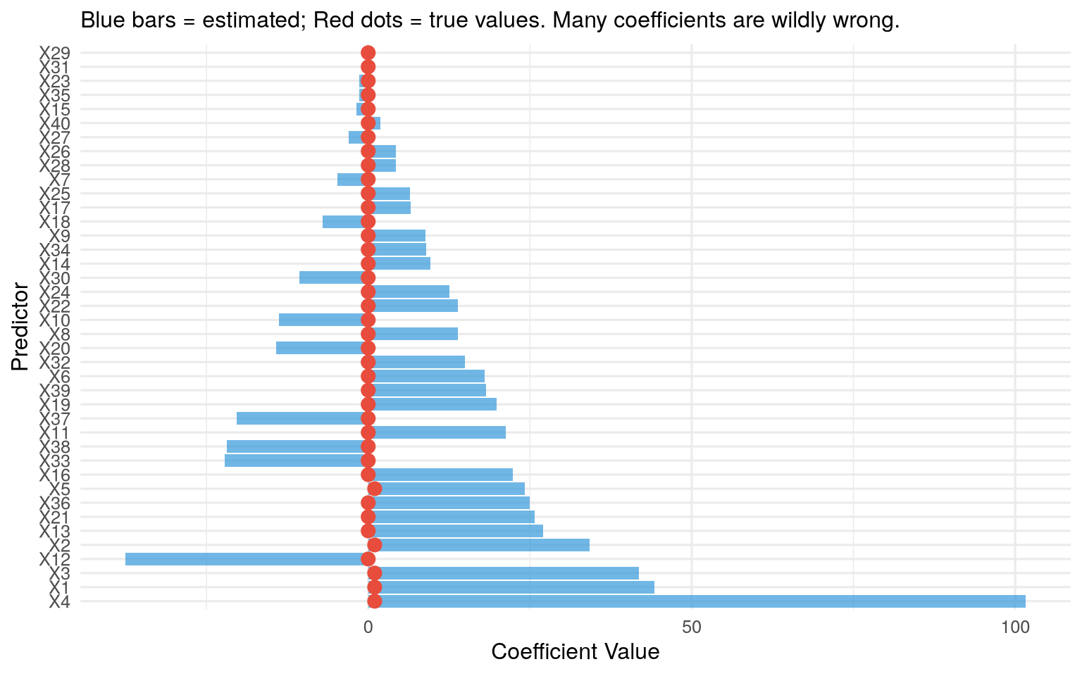
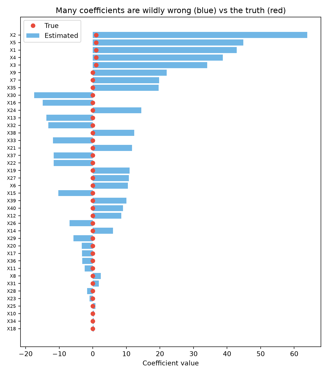
To make the problem concrete, the simulation below creates a dataset where we *know* the truth: 100 patients, 40 candidate predictors, but only the first 5 actually influence the outcome (the other 35 are pure noise with a true coefficient of zero). We then fit a standard logistic regression and compare the coefficients it estimates (blue bars) against the true values (red dots). If the method were working well, the blue bars should sit near the red dots --- near zero for the 35 noise predictors. Instead, because there are far too many predictors for the available information, many coefficients are estimated as large positive or negative values for variables that have *no real effect at all*. That is overfitting made visible: the model is fitting the noise.
::: {.panel-tabset}
#### R
```{r}
#| label: fig-overfitting-demo
#| fig-cap: "Simulated example: standard logistic regression with 40 predictors and 100 observations. Many coefficients are wildly inflated. True coefficients (most are zero) are shown in red."
#| code-fold: true
#| warning: false
#| message: false
library(ggplot2)

set.seed(42)
n <- 100
p <- 40

# True model: only 5 predictors matter
X <- matrix(rnorm(n * p), n, p)
colnames(X) <- paste0("X", 1:p)
true_beta <- c(rep(1, 5), rep(0, p - 5))
logit_p <- X %*% true_beta
y <- rbinom(n, 1, plogis(logit_p))

# Fit standard logistic regression (suppress warnings about non-convergence)
fit_standard <- suppressWarnings(
  glm(y ~ X, family = binomial())
)

coef_df <- data.frame(
  predictor = paste0("X", 1:p),
  estimated = coef(fit_standard)[-1], # Remove intercept
  true = true_beta
)

ggplot(coef_df, aes(x = reorder(predictor, -abs(estimated)))) +
  geom_col(aes(y = estimated), fill = "#3498db", alpha = 0.7) +
  geom_point(aes(y = true), colour = "#e74c3c", size = 3) +
  coord_flip() +
  labs(
    x = "Predictor",
    y = "Coefficient Value",
    subtitle = "Blue bars = estimated; Red dots = true values. Many coefficients are wildly wrong."
  ) +
  theme_minimal(base_size = 12)
```
#### Python
```{python}
#| label: fig-overfitting-demo-python
#| fig-cap: "The same demonstration in Python: standard logistic regression with 40 predictors and 100 observations. Estimated coefficients (blue) bear little resemblance to the true values (red dots)."
#| code-fold: true
#| warning: false
#| message: false
import numpy as np
import matplotlib.pyplot as plt
from sklearn.linear_model import LogisticRegression

rng = np.random.default_rng(42)
n, p = 100, 40

# True model: only the first 5 predictors matter
X = rng.normal(size=(n, p))
true_beta = np.array([1.0] * 5 + [0.0] * (p - 5))
y = rng.binomial(1, 1 / (1 + np.exp(-(X @ true_beta))))

# Standard (essentially unpenalised) logistic regression
fit = LogisticRegression(penalty=None, max_iter=10000).fit(X, y)
estimated = fit.coef_[0]

order = np.argsort(np.abs(estimated))
plt.figure(figsize=(7, 8))
plt.barh(range(p), estimated[order], color="#3498db", alpha=0.7, label="Estimated")
plt.plot(true_beta[order], range(p), "o", color="#e74c3c", label="True")
plt.yticks(range(p), [f"X{j+1}" for j in order], fontsize=7)
plt.xlabel("Coefficient value")
plt.title("Many coefficients are wildly wrong (blue) vs the truth (red)")
plt.legend(loc="best")
plt.tight_layout()
plt.show()
```
:::
## The Bias-Variance Tradeoff
The fundamental insight behind penalised regression is the **bias-variance tradeoff**.
### Prediction Error Decomposition
The expected prediction error of a model can be decomposed into three components:
$$\text{Expected Error} = \text{Bias}^2 + \text{Variance} + \text{Irreducible Noise}$$
- **Bias** is the systematic error introduced by simplifying assumptions. A model that is too simple (e.g., a linear model for a non-linear relationship) has high bias.
- **Variance** is the sensitivity of the model to the specific training data. A model that is too complex (e.g., 50 predictors with 40 events) has high variance.
- **Irreducible noise** is the inherent randomness in the outcome that no model can capture.
### The Tradeoff
Standard regression (OLS, maximum likelihood) is **unbiased** --- meaning that if you could repeat your study many times on fresh samples and average the coefficient estimates, that average would land on the true value. There is no systematic tendency to over- or under-estimate. (This is a guaranteed mathematical property of least squares and maximum likelihood under the usual modelling assumptions; it is *why* these methods are the default starting point.) But notice what "unbiased on average" does *not* promise: that any *single* estimate from your *one* actual dataset is close to the truth. In high-dimensional or small-sample settings, the estimates scatter enormously from sample to sample --- they are correct on average but wildly imprecise in any given sample. That scatter is the variance, and it is what penalisation attacks.
Penalised regression deliberately introduces a small amount of bias --- shrinking coefficients toward zero --- in exchange for a dramatic reduction in variance. The net effect is a model with **lower total prediction error** despite being biased.
Think of it this way: if the true coefficient is 0.5, an unbiased estimator might give you estimates of -2.3, 3.1, 0.8, -1.5, etc. across different samples (unbiased on average, but highly variable). A biased estimator that consistently gives you 0.3 is much closer to the truth in any given sample, even though it is systematically too low.
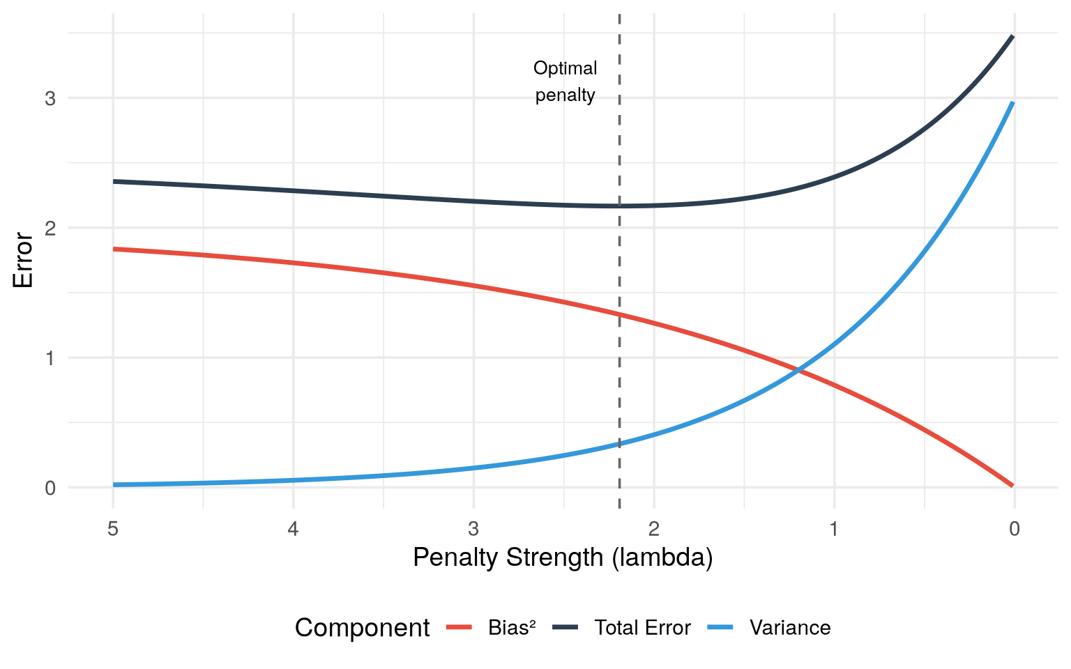
The figure below makes this tradeoff visual. The horizontal axis is the penalty strength $\lambda$, plotted so that the penalty *increases* as you move to the right (equivalently, model complexity *decreases* to the right). Watch the three curves as the penalty grows: **bias²** (red) rises, because shrinking coefficients toward zero introduces systematic error; **variance** (blue) falls, because a more constrained model is less sensitive to the particular sample; and the **total error** (dark line), which is their sum plus irreducible noise, is U-shaped. The dashed vertical line marks the sweet spot --- the penalty that minimises total error. Too little penalty (far left) and variance dominates; too much (far right) and bias dominates. Cross-validation, introduced later, is simply an automatic way to find that dashed line from data.
```{r}
#| label: fig-bias-variance
#| fig-cap: "The bias-variance tradeoff. As model complexity increases (or penalty decreases), bias decreases but variance increases. The sweet spot minimises total error."
#| code-fold: true
#| warning: false
library(ggplot2)

lambda <- seq(0.01, 5, length.out = 200)
bias2 <- 2 * (1 - exp(-0.5 * lambda))
variance <- 3 * exp(-lambda)
total <- bias2 + variance + 0.5

df_bv <- data.frame(
  lambda = rep(lambda, 3),
  error = c(bias2, variance, total),
  component = rep(c("Bias²", "Variance", "Total Error"), each = length(lambda))
)

ggplot(df_bv, aes(x = lambda, y = error, colour = component)) +
  geom_line(linewidth = 1.2) +
  scale_colour_manual(
    values = c(
      "Bias²" = "#e74c3c",
      "Variance" = "#3498db",
      "Total Error" = "#2c3e50"
    )
  ) +
  geom_vline(
    xintercept = lambda[which.min(total)],
    linetype = "dashed",
    colour = "grey40"
  ) +
  annotate(
    "text",
    x = lambda[which.min(total)] + 0.3,
    y = max(total) * 0.9,
    label = "Optimal\npenalty",
    size = 3.5
  ) +
  labs(x = "Penalty Strength (lambda)", y = "Error", colour = "Component") +
  scale_x_reverse() +
  theme_minimal(base_size = 14) +
  theme(legend.position = "bottom")
```
## The Penalised Regression Framework
### The General Idea
In standard regression, we estimate coefficients by minimising a loss function (e.g., residual sum of squares for linear regression, negative log-likelihood for logistic regression):
$$\hat{\boldsymbol{\beta}} = \arg\min_{\boldsymbol{\beta}} \left\{ \text{Loss}(\boldsymbol{\beta}) \right\}$$
In penalised regression, we add a **penalty term** that grows with the size of the coefficients:
$$\hat{\boldsymbol{\beta}} = \arg\min_{\boldsymbol{\beta}} \left\{ \text{Loss}(\boldsymbol{\beta}) + \lambda \cdot \text{Penalty}(\boldsymbol{\beta}) \right\}$$
The penalty term discourages large coefficients. The tuning parameter $\lambda \geq 0$ controls the strength of the penalty:
- $\lambda = 0$: no penalty, equivalent to standard regression
- $\lambda \to \infty$: all coefficients shrunk to zero (null model)
- Intermediate $\lambda$: the sweet spot, chosen by cross-validation
We will lean on **cross-validation** repeatedly to choose $\lambda$, so here is the idea in one sentence (it gets a full treatment in @sec-choosing-lambda): cross-validation repeatedly hides part of the data, fits the model on the rest, and checks how well it predicts the hidden part --- giving an honest estimate of out-of-sample performance for each candidate $\lambda$, so we can pick the value that predicts best on data the model has not seen.
The three main methods differ only in the form of the penalty.
::: {.callout-important}
## Standardisation Is Essential
Before applying penalised regression, all predictors must be **standardised**. Standardising a variable means two simple steps: subtract its mean (so the new variable is centred at zero) and divide by its standard deviation (so a one-unit change now means "one standard deviation"). For a predictor $x_j$ with mean $\bar{x}_j$ and standard deviation $s_j$, each value becomes
$$z_{ij} = \frac{x_{ij} - \bar{x}_j}{s_j}.$$
After this, every predictor is on the same footing: mean zero, standard deviation one, no units.
Why does this matter here specifically? The penalty adds up the sizes of the coefficients ($\sum \beta_j^2$ for ridge, $\sum |\beta_j|$ for LASSO) and treats every coefficient the same way. But a coefficient's size depends on the units of its predictor. Measure a drug dose in milligrams and the coefficient is small; measure the *same* dose in kilograms and the coefficient is a million times larger --- even though nothing about the science changed. Because the penalty only "sees" coefficient size, it would shrink the kilogram version far more aggressively than the milligram version. Standardising removes this arbitrariness, so the penalty reflects each predictor's genuine contribution rather than the accident of its measurement scale.
Both `glmnet` (R) and `sklearn` (Python) standardise internally by default and then report coefficients back on the original scale, so you usually do not have to do this by hand --- but you should know it is happening, because it explains why penalised coefficients are not directly comparable to ordinary regression coefficients unless you account for it.
:::
## Ridge Regression (L2 Penalty)
### Definition
Ridge regression, introduced by Hoerl and Kennard [-@hoerl1970], adds the **squared sum of coefficients** (L2 norm) as the penalty:
$$\hat{\boldsymbol{\beta}}_{\text{Ridge}} = \arg\min_{\boldsymbol{\beta}} \left\{ \underbrace{\sum_{i=1}^{n} \left( y_i - \beta_0 - \sum_{j=1}^{p} \beta_j x_{ij} \right)^2}_{\text{(1) how badly the model fits the data}} + \underbrace{\lambda \sum_{j=1}^{p} \beta_j^2}_{\text{(2) penalty for large coefficients}} \right\}$$
The equation looks dense, but it is saying something simple. Read it as a tug-of-war between two quantities the model tries to keep small at the same time:
- **Term (1) — misfit.** This is the ordinary regression criterion: for each patient $i$, take the gap between the observed outcome $y_i$ and the model's prediction, square it, and add up over all patients. Smaller means the model fits the data better. On its own, minimising this term is just standard regression.
- **Term (2) — penalty.** This adds up the squared coefficients and multiplies by $\lambda$. It grows whenever coefficients get large, so it pushes them back toward zero. $\lambda$ is the dial that sets how strong that pushback is.
"$\arg\min_{\boldsymbol{\beta}}$" just means *find the set of coefficients $\boldsymbol{\beta}$ that makes the whole expression as small as possible*. So ridge regression looks for coefficients that fit the data well **and** stay modest in size, with $\lambda$ deciding how much weight to give each goal. Set $\lambda = 0$ and the penalty vanishes, recovering ordinary regression; make $\lambda$ very large and the coefficients are squeezed close to zero.
Note that the **intercept** $\beta_0$ is typically **not penalised** --- only the predictor coefficients $\beta_1, \ldots, \beta_p$ are shrunk, because the intercept just sets the baseline level of the outcome and shrinking it would have no useful effect.
### Key Properties
Ridge has three properties worth understanding. The first is the one that matters most in practice; the other two explain *why* ridge is so well-behaved.
1. **It shrinks every coefficient toward zero, but never all the way to zero.** No matter how strong the penalty, ridge makes coefficients smaller without ever switching any off completely --- they get tiny, but stay non-zero. The practical upshot is that ridge keeps *all* of your predictors in the model.
This is the place to define a term used throughout the chapter. **Variable selection** means automatically deciding which predictors to *keep* and which to *drop entirely* from the model --- in effect, setting some coefficients to exactly zero so those variables disappear. It is what you would otherwise do by hand when you trim a model down to a short, usable list of predictors. **Ridge does not do variable selection**: because its coefficients never hit exactly zero, every predictor stays in, just with a reduced weight. (The LASSO, covered next, *does* perform variable selection --- this is the single biggest difference between the two methods, so keep the contrast in mind.)
2. **It has a closed-form solution.** "Closed-form" means the answer can be computed directly with a single formula, rather than by an iterative search. For ridge that formula is:
$$\hat{\boldsymbol{\beta}}_{\text{Ridge}} = (\mathbf{X}^T\mathbf{X} + \lambda \mathbf{I})^{-1} \mathbf{X}^T \mathbf{y}$$
You do not need to manipulate this by hand --- the software does. The point to take away is the role of the $\lambda \mathbf{I}$ piece: adding it guarantees the matrix can always be inverted (i.e., the equation always has a unique, stable solution), even when there are more predictors than patients ($p > n$) or when predictors are highly correlated --- exactly the cases where ordinary regression fails. This is the mathematical reason ridge "rescues" problems that would otherwise have no stable answer.
3. **It handles multicollinearity gracefully.** *Multicollinearity* is when predictors carry overlapping information --- systolic and diastolic blood pressure, or several related inflammatory markers. Ordinary regression reacts badly to this: it cannot decide how to split the shared effect between the correlated variables, so it produces wildly unstable coefficients that can even come out with the wrong sign. Ridge calms this down by pulling correlated predictors toward a shared, modest value instead of letting them swing against each other.
### When to Use Ridge
- You believe **many predictors** contribute to the outcome (none is truly zero)
- Predictors are **highly correlated** (multicollinearity)
- You care about **prediction accuracy** more than variable selection
- Example: predicting ICU mortality using dozens of physiological measurements, most of which carry some information
## LASSO Regression (L1 Penalty)
### Definition
The LASSO (Least Absolute Shrinkage and Selection Operator), introduced by Tibshirani [-@tibshirani1996], uses the **sum of absolute values** (L1 norm) as the penalty:
$$\hat{\boldsymbol{\beta}}_{\text{LASSO}} = \arg\min_{\boldsymbol{\beta}} \left\{ \sum_{i=1}^{n} \left( y_i - \beta_0 - \sum_{j=1}^{p} \beta_j x_{ij} \right)^2 + \lambda \sum_{j=1}^{p} |\beta_j| \right\}$$
### Key Properties
1. **Shrinks some coefficients to exactly zero.** This is the defining feature of the LASSO. When $\lambda$ is large enough, some coefficients are forced to zero, effectively removing those predictors from the model. The LASSO thus performs **automatic variable selection**.
2. **No closed-form solution.** Unlike Ridge, the LASSO requires iterative optimisation algorithms (coordinate descent is the standard approach in `glmnet`).
3. **Selects at most $n$ predictors** (when $p > n$). The LASSO can select at most $\min(n, p)$ predictors. When you have far more predictors than observations, this is a useful property.
4. **Struggles with correlated predictors.** When two predictors are highly correlated, the LASSO tends to pick one and drop the other arbitrarily. This can lead to **unstable variable selection** --- which predictor is kept can change across different samples.
### Why Sparsity Matters Clinically
In clinical research, we often want to identify the **most important predictors** from a larger set of candidates. This is common in:
- **Clinical prediction model development.** A parsimonious model with 5--10 predictors is more practical than one with 50.
- **Biomarker discovery.** From a panel of 100 candidate biomarkers, which ones are truly associated with the outcome?
- **Risk factor identification.** Among many potential lifestyle, genetic, and environmental factors, which are the strongest?
The LASSO's ability to set coefficients exactly to zero makes it a natural tool for these tasks.
::: {.callout-warning}
## LASSO Is Not a Substitute for Domain Knowledge
While the LASSO performs automatic variable selection, the results should always be interpreted in light of clinical knowledge. A variable dropped by the LASSO is not necessarily unimportant --- it may be correlated with another retained variable, or the sample may be too small to detect its effect. Similarly, a variable retained by the LASSO is not necessarily causal.
Use the LASSO as a tool to *complement*, not replace, clinical reasoning about which variables matter.
:::
## Elastic Net: The Best of Both Worlds
### Definition
The Elastic Net, proposed by Zou and Hastie [-@zou2005], combines both L1 and L2 penalties:
$$\hat{\boldsymbol{\beta}}_{\text{EN}} = \arg\min_{\boldsymbol{\beta}} \left\{ \text{Loss}(\boldsymbol{\beta}) + \lambda \left[ \alpha \sum_{j=1}^{p} |\beta_j| + \frac{(1-\alpha)}{2} \sum_{j=1}^{p} \beta_j^2 \right] \right\}$$
The parameter $\alpha \in [0, 1]$ controls the **mix** of L1 and L2:
- $\alpha = 1$: pure LASSO
- $\alpha = 0$: pure Ridge
- $0 < \alpha < 1$: Elastic Net (a blend)
### Why Combine?
The Elastic Net addresses the LASSO's limitations while retaining its strengths:
1. **Correlated predictors.** When predictors are correlated, the LASSO picks one and drops the rest. The Elastic Net tends to **keep correlated predictors together** (the "grouping effect"), either including all of them or excluding all of them. This is often more scientifically reasonable.
2. **More than $n$ predictors.** The LASSO selects at most $n$ predictors. The Elastic Net can select more, which is useful in genomics where thousands of genes may be relevant.
3. **Stability.** The Elastic Net generally produces more stable results than the LASSO across different samples.
### Choosing Alpha
In practice, $\alpha$ is often chosen by **cross-validation** alongside $\lambda$. Cross-validation (defined fully in @sec-choosing-lambda) is the standard tool for choosing *any* tuning parameter: it scores each candidate value by how well the resulting model predicts data it was not trained on. Here we have two dials to set --- $\alpha$ (the L1/L2 mix) and $\lambda$ (the overall strength) --- so we search over a grid of both:
- Try $\alpha \in \{0.1, 0.25, 0.5, 0.75, 0.9, 1.0\}$
- For each $\alpha$, use cross-validation to find the optimal $\lambda$ (this is the inner search `cv.glmnet` does automatically)
- Select the $(\alpha, \lambda)$ combination with the best cross-validated performance
In practice this is a short loop over the $\alpha$ values, calling cross-validation once per $\alpha$ and keeping the best pair --- exactly the pattern shown in the R implementation walkthrough later in this chapter. If you would rather not search at all, $\alpha = 0.5$ is a reasonable default that balances L1 and L2 equally and works well in many clinical datasets.
## Choosing Lambda: Cross-Validation {#sec-choosing-lambda}
### The Cross-Validation Procedure
The tuning parameter $\lambda$ controls the penalty strength. We cannot estimate it from the data using the same approach as the regression coefficients --- it must be chosen externally. **K-fold cross-validation** is the standard approach:
1. Divide the data into $K$ folds (typically $K = 10$).
2. For each value of $\lambda$ on a grid:
a. For each fold, fit the model on the other $K-1$ folds and predict the held-out fold.
b. Calculate the prediction error (e.g., mean squared error, deviance, or misclassification rate).
3. Average the prediction error across folds for each $\lambda$.
4. Select the $\lambda$ that minimises the average prediction error.
### Lambda.min vs Lambda.1se
Cross-validation typically identifies two candidate values of $\lambda$:
- **lambda.min**: the value of $\lambda$ that minimises the cross-validated error. This gives the model with the best predictive performance.
- **lambda.1se**: the largest $\lambda$ whose cross-validated error is within one standard error of the minimum. This gives a **simpler, more parsimonious model** that is nearly as good as the best.
::: {.callout-tip}
## Which Lambda to Use?
In clinical prediction modelling, `lambda.min` is often preferred when predictive accuracy is the primary goal. In biomarker discovery or variable selection, `lambda.1se` is often preferred because it gives a more parsimonious model with fewer selected variables.
Steyerberg [-@steyerberg2019] recommends reporting results for both and discussing the trade-off between parsimony and performance.
:::
```{r}
#| label: fig-cv-lambda
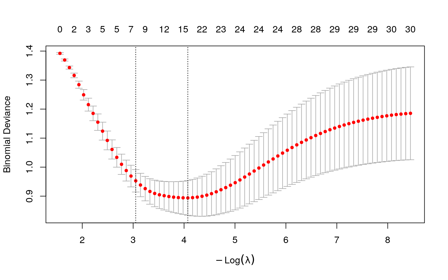
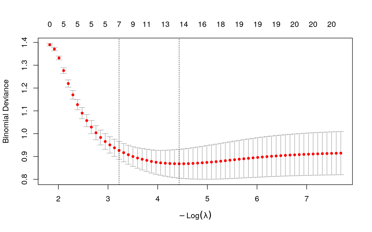
#| fig-cap: "Cross-validation curve for LASSO. The x-axis is -log(lambda) (so the penalty decreases left to right), the y-axis is cross-validated deviance. Vertical lines mark lambda.1se (left) and lambda.min (right)."
#| code-fold: true
#| warning: false
#| message: false
library(glmnet)

set.seed(42)
n <- 200
p <- 30
X <- matrix(rnorm(n * p), n, p)
true_beta <- c(rep(1.5, 5), rep(0, 25))
y <- rbinom(n, 1, plogis(X %*% true_beta))

cv_fit <- cv.glmnet(X, y, family = "binomial", alpha = 1, nfolds = 10)
plot(cv_fit)
```
**How to read this plot.** This is the standard `glmnet` cross-validation plot, and it repays a careful look. One orientation point first: current versions of `glmnet` label the x-axis $-\log(\lambda)$ (negative log lambda), so the penalty *decreases* from left to right. This is the opposite layout to a plain $\log(\lambda)$ axis, so read it carefully:
- The **x-axis** is $-\log(\lambda)$. Because of the minus sign, the penalty is *strongest* on the **left** (large $\lambda$, a heavily shrunk model) and *weakest* on the **right** (small $\lambda$, a complex model close to ordinary regression). Each red dot is one candidate $\lambda$.
- The **y-axis** is the cross-validated **deviance** --- a measure of prediction error (lower is better; see the deviance explanation later in this chapter). Each red dot is the average error across the 10 folds for that $\lambda$, and the **vertical bars** through it show ±1 standard error of that average, i.e. how uncertain the estimate is.
- The numbers along the **top** count how many predictors remain in the model (have non-zero coefficients) at each $\lambda$ --- notice they *grow* from left to right (few on the strongly-penalised left, all of them on the weakly-penalised right) as the penalty releases more coefficients from zero.
- The two **dashed vertical lines** mark the two recommended choices. Because larger $\lambda$ is now on the left, `lambda.1se` (the largest $\lambda$ within one standard error of the best --- the simpler, more parsimonious model) is the **left** line, and `lambda.min` (the $\lambda$ with the lowest average error) is the **right** line.
So the plot is really a picture of the bias-variance tradeoff from earlier, drawn from real cross-validated data: error is high when the penalty is too strong (over-shrinking, far left) *and* when it is too weak (overfitting, far right), with a basin of good values in between that the two dashed lines bracket.
## Regularisation Paths
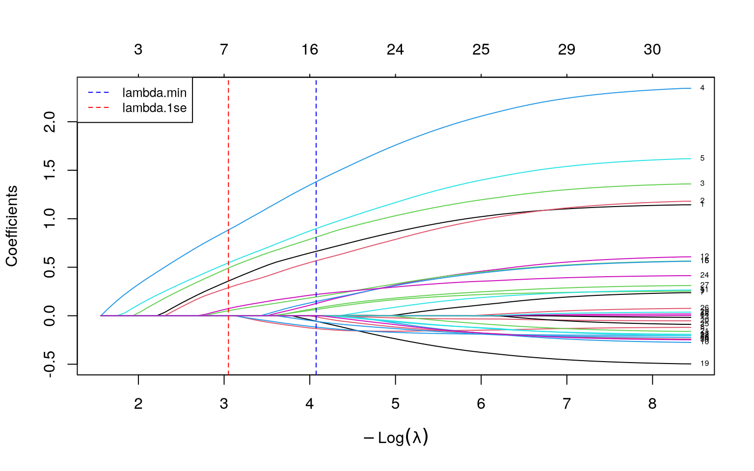
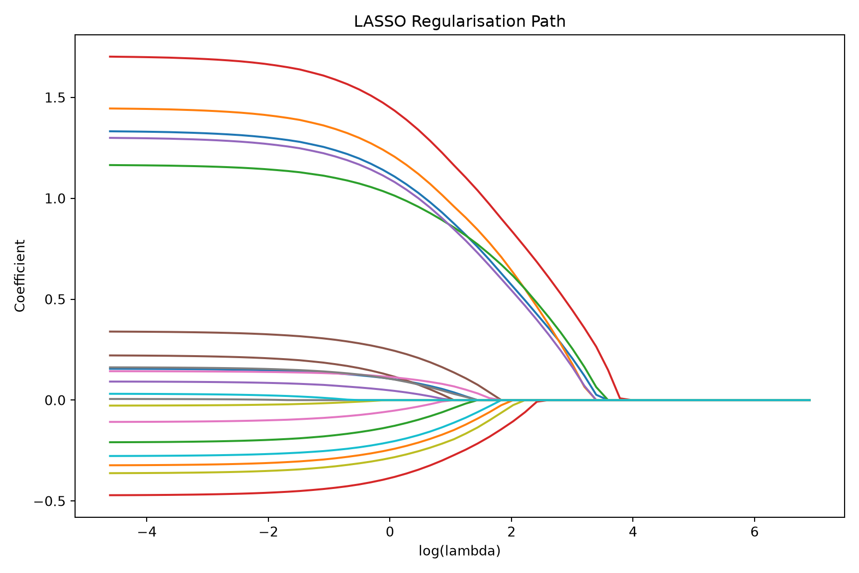
A **regularisation path** (also called a coefficient trace or coefficient path) shows how each coefficient changes as $\lambda$ varies from large (strong penalty) to small (weak penalty).
The code below fits a LASSO over the *whole range* of $\lambda$ in one call (`glmnet` does this automatically --- you do not specify a single $\lambda$), then plots every coefficient as a line. The two dashed vertical lines reuse the `lambda.min` and `lambda.1se` values found by cross-validation in the previous section, so you can see which coefficients survive at each recommended penalty. On the $-\log(\lambda)$ axis the penalty relaxes as you move left to right, so you watch predictors switch on one by one from left (strong penalty, all near zero) to right (weak penalty, all active).
```{r}
#| label: fig-regularisation-path
#| fig-cap: "LASSO regularisation path. Each line is one coefficient. As lambda decreases (left to right), more coefficients become non-zero. The five truly non-zero coefficients (shown as they enter the model) are recovered first."
#| code-fold: true
#| warning: false
#| message: false
library(glmnet)

fit_lasso <- glmnet(X, y, family = "binomial", alpha = 1)
# glmnet 5.0 draws this plot on a -log(lambda) axis, so the reference
# lines are placed at -log(lambda.min) and -log(lambda.1se) to match.
plot(fit_lasso, xvar = "lambda", label = TRUE)
abline(v = -log(cv_fit$lambda.min), lty = 2, col = "blue")
abline(v = -log(cv_fit$lambda.1se), lty = 2, col = "red")
legend(
  "topleft",
  legend = c("lambda.min", "lambda.1se"),
  col = c("blue", "red"),
  lty = 2,
  cex = 0.8
)
```
### How to Read a Regularisation Path
First, the x-axis. Current `glmnet` (version 5.0 and later) labels it $-\log(\lambda)$ --- *negative* log lambda. The minus sign matters: it means the penalty *decreases* as you move from left to right. So large penalties sit on the **left** and small penalties on the **right** --- the mirror image of a plain $\log(\lambda)$ axis. This is the same axis as the cross-validation plot in the previous section, so the two figures line up. (If you have seen older `glmnet` figures with a $\log(\lambda)$ axis, the left--right orientation there is reversed; always read the axis label.)
With that settled, here is how to read the curves:
- **Left side** (large $\lambda$, small $-\log\lambda$): strong penalty, all coefficients squeezed to near zero.
- **Right side** (small $\lambda$, large $-\log\lambda$): weak penalty, coefficients approach their ordinary (unpenalised) regression values.
- **Order of entry**: predictors whose lines peel away from zero **earliest --- i.e. furthest to the left, while the penalty is still strong** --- are the most important, because they survive the heaviest shrinkage.
- **Sign and magnitude**: the sign and eventual magnitude of each line reveal the direction and strength of that predictor's association.
The two dashed vertical lines mark the cross-validated `lambda.min` and `lambda.1se`, so you can read off which coefficients are non-zero at each recommended penalty. This plot is extremely useful for understanding the relative importance of predictors and the stability of the model across different penalty strengths.
## Clinical Example: Breast Cancer Diagnosis from Image Features
### The Dataset
The Original Wisconsin Breast Cancer dataset (the `BreastCancer` data in the `mlbench` package, used in the code below) contains 699 biopsy samples scored on **9 cytological attributes**, each graded 1--10 by a pathologist: clump thickness, uniformity of cell size, uniformity of cell shape, marginal adhesion, single epithelial cell size, bare nuclei, bland chromatin, normal nucleoli, and mitoses. The outcome is the diagnosis: malignant or benign.
With 9 predictors and several hundred observations, this is not a $p > n$ problem, but it is still a useful setting for penalised regression because many of the cytological features are highly correlated (cell-size and cell-shape uniformity, for instance, tend to move together). Correlated predictors are exactly where the three methods behave differently, which is what makes the comparison below instructive.
::: {.callout-note}
## What is "deviance"?
The code below reports model performance as **deviance**, a term that recurs whenever we fit logistic (and other generalised linear) models, so it is worth pinning down. Deviance is a measure of **how poorly a model fits**, built from the likelihood: it is defined as $-2 \times$ the log-likelihood of the fitted model. Lower deviance means a better fit. For ordinary linear regression, deviance reduces to the residual sum of squares, so you can think of it as the natural extension of "squared prediction error" to logistic regression and other models where squared error does not directly apply. When we report **cross-validated deviance**, we mean the deviance computed on held-out folds --- so it measures how well the model predicts *new* data, not how well it memorised the training data. It is the default error measure `glmnet` minimises when choosing $\lambda$ for a binary outcome.
:::
The worked example below is shown in both R (`glmnet`) and Python (`scikit-learn`). Both fit LASSO, Ridge, and Elastic Net to the same kind of problem and compare the resulting coefficients; the datasets shipped with each language differ slightly (R's `mlbench` carries the 9-attribute Original Wisconsin data; scikit-learn ships the 30-feature Diagnostic version), so the exact numbers differ, but the *pattern* is identical and is the point of the example.
::: {.panel-tabset}
#### R
```{r}
#| label: breast-cancer-r
#| warning: false
#| message: false
library(glmnet)
library(ggplot2)

# Load the dataset (9 cytological attributes, Original Wisconsin data)
# install.packages("mlbench")
data(BreastCancer, package = "mlbench")

# Prepare the data
bc <- BreastCancer[complete.cases(BreastCancer), ]
bc$diagnosis <- ifelse(bc$Class == "malignant", 1, 0)

# Extract numeric predictors (the 9 cytological attributes, columns 2-10)
X <- as.matrix(apply(bc[, 2:10], 2, as.numeric))
y <- bc$diagnosis

# Fit LASSO with cross-validation
set.seed(42)
cv_lasso <- cv.glmnet(X, y, family = "binomial", alpha = 1, nfolds = 10)

# Compare LASSO, Ridge, and Elastic Net
set.seed(42)
cv_ridge <- cv.glmnet(X, y, family = "binomial", alpha = 0, nfolds = 10)
cv_enet <- cv.glmnet(X, y, family = "binomial", alpha = 0.5, nfolds = 10)

# The two standard LASSO penalties chosen by cross-validation
lambda_tab <- data.frame(
  Choice = c("lambda.min (best prediction)", "lambda.1se (parsimonious)"),
  Lambda = round(c(cv_lasso$lambda.min, cv_lasso$lambda.1se), 4)
)
knitr::kable(
  lambda_tab,
  caption = "The two standard LASSO penalties chosen by cross-validation."
)

# LASSO coefficients (log-odds scale) at each penalty
coef_1se <- as.matrix(coef(cv_lasso, s = "lambda.1se"))
coef_min <- as.matrix(coef(cv_lasso, s = "lambda.min"))
coef_tab <- data.frame(
  Variable = rownames(coef_1se),
  `lambda.1se` = round(coef_1se[, 1], 4),
  `lambda.min` = round(coef_min[, 1], 4),
  check.names = FALSE,
  row.names = NULL
)
# keep only variables retained by at least one penalty
coef_tab <- coef_tab[
  coef_tab[["lambda.1se"]] != 0 | coef_tab[["lambda.min"]] != 0,
]
knitr::kable(
  coef_tab,
  caption = "LASSO coefficients (log-odds scale) at each penalty. A zero means the variable was shrunk out of the model."
)

# Cross-validated deviance for the three methods (lower = better fit)
deviance_tab <- data.frame(
  Method = c("Ridge", "Elastic Net", "LASSO"),
  `CV deviance` = round(
    c(min(cv_ridge$cvm), min(cv_enet$cvm), min(cv_lasso$cvm)),
    4
  ),
  check.names = FALSE
)
knitr::kable(
  deviance_tab,
  caption = "Cross-validated deviance at lambda.min (lower = better fit)."
)
```
```{r}
#| label: fig-compare-methods
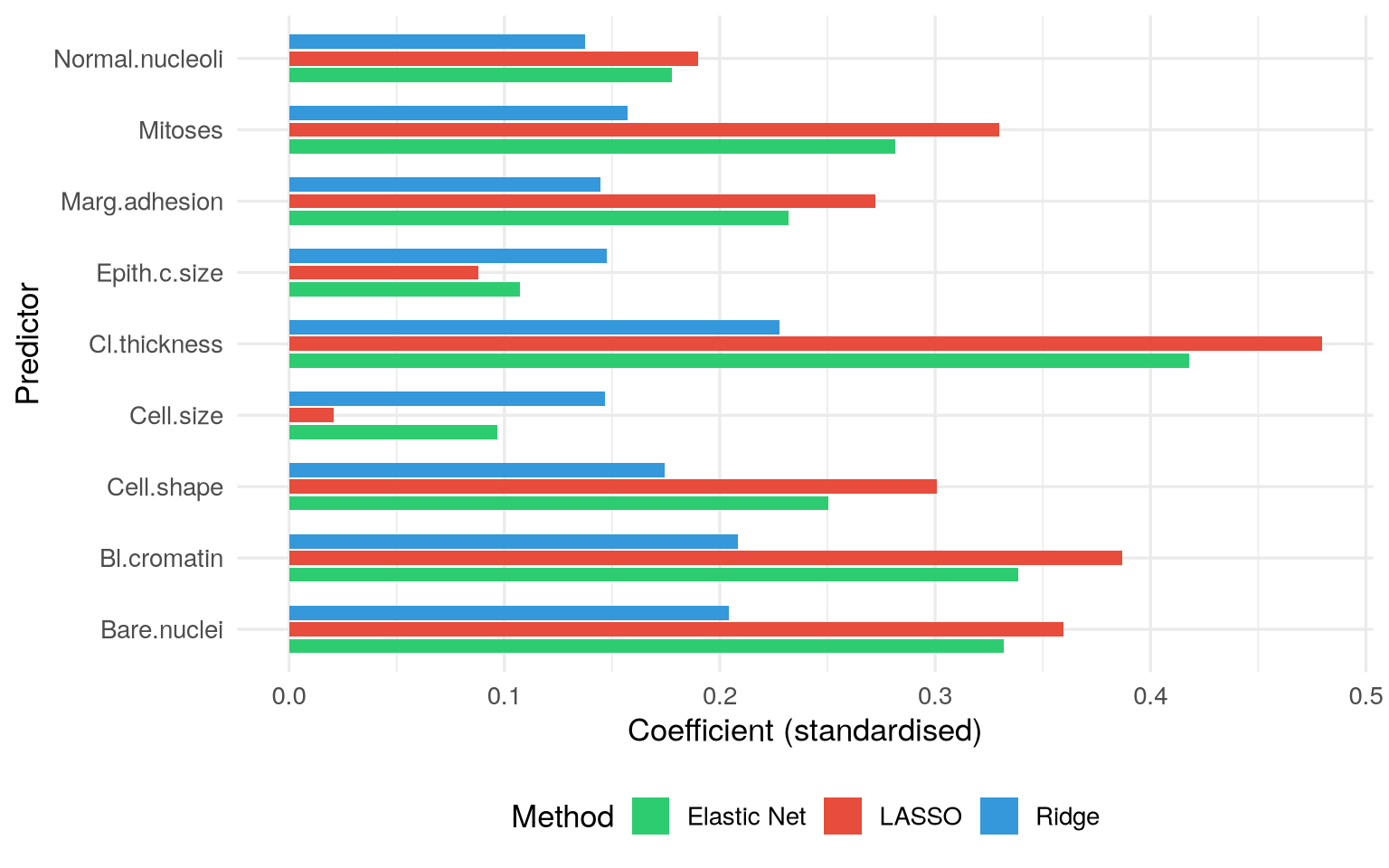
#| fig-cap: "Coefficient estimates from Ridge, Elastic Net, and LASSO for the breast cancer dataset (R). Ridge retains all predictors; LASSO sets some to zero; Elastic Net is intermediate."
#| code-fold: true
#| warning: false
#| message: false
library(tidyverse)   # ggplot2 / dplyr / tibble

# Extract coefficients at lambda.min for each method
coef_ridge <- as.vector(coef(cv_ridge, s = "lambda.min"))[-1]
coef_enet <- as.vector(coef(cv_enet, s = "lambda.min"))[-1]
coef_lasso <- as.vector(coef(cv_lasso, s = "lambda.min"))[-1]

pred_names <- colnames(X)

comp_df <- data.frame(
  predictor = rep(pred_names, 3),
  coefficient = c(coef_ridge, coef_enet, coef_lasso),
  method = rep(c("Ridge", "Elastic Net", "LASSO"), each = length(pred_names))
)

ggplot(comp_df, aes(x = predictor, y = coefficient, fill = method)) +
  geom_col(position = position_dodge(width = 0.7), width = 0.6) +
  scale_fill_manual(
    values = c(
      "Ridge" = "#3498db",
      "Elastic Net" = "#2ecc71",
      "LASSO" = "#e74c3c"
    )
  ) +
  coord_flip() +
  labs(x = "Predictor", y = "Coefficient (standardised)", fill = "Method") +
  theme_minimal(base_size = 13) +
  theme(legend.position = "bottom")
```
#### Python
```{python}
#| label: breast-cancer-python
#| output: false
#| warning: false
#| message: false
import numpy as np
import pandas as pd
import matplotlib.pyplot as plt
from sklearn.datasets import load_breast_cancer
from sklearn.preprocessing import StandardScaler
from sklearn.linear_model import LogisticRegressionCV

# scikit-learn ships the 30-feature Diagnostic version of the dataset
data = load_breast_cancer()
X = StandardScaler().fit_transform(data.data)
y = data.target  # 1 = benign, 0 = malignant in sklearn's coding
feature_names = data.feature_names

# Fit LASSO, Ridge, and Elastic Net, each tuned by cross-validation
# In sklearn, C = 1/lambda, so it tunes C; penalty selects the norm
common = dict(Cs=20, cv=10, scoring="neg_log_loss",
              max_iter=10000, random_state=42)
lasso = LogisticRegressionCV(penalty="l1", solver="saga", **common).fit(X, y)
ridge = LogisticRegressionCV(penalty="l2", solver="lbfgs", **common).fit(X, y)
enet = LogisticRegressionCV(penalty="elasticnet", solver="saga",
                            l1_ratios=[0.5], **common).fit(X, y)

n_lasso = int(np.sum(np.abs(lasso.coef_[0]) > 1e-6))
n_ridge = int(np.sum(np.abs(ridge.coef_[0]) > 1e-6))
n_enet = int(np.sum(np.abs(enet.coef_[0]) > 1e-6))
print(f"Non-zero coefficients (of {X.shape[1]}):")
print(f" Ridge: {n_ridge}")
print(f" Elastic Net: {n_enet}")
print(f" LASSO: {n_lasso}")
```
```{python}
#| label: fig-compare-methods-python
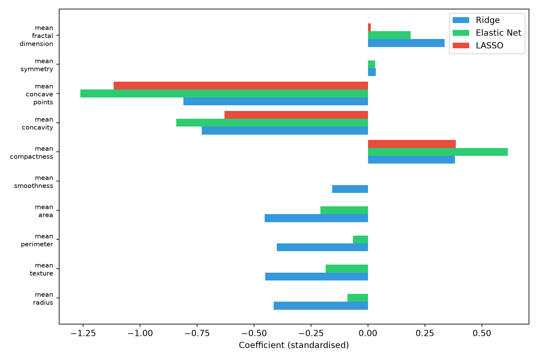
#| fig-cap: "Coefficient estimates from Ridge, Elastic Net, and LASSO for the breast cancer dataset (Python). Ridge retains all predictors; LASSO sets many to zero; Elastic Net is intermediate."
#| code-fold: true
#| warning: false
#| message: false
# Show the first 10 features for legibility
k = 10
idx = np.arange(k)
width = 0.27

plt.figure(figsize=(9, 6))
plt.barh(idx - width, ridge.coef_[0][:k], height=width, label="Ridge", color="#3498db")
plt.barh(idx, enet.coef_[0][:k], height=width, label="Elastic Net", color="#2ecc71")
plt.barh(idx + width, lasso.coef_[0][:k], height=width, label="LASSO", color="#e74c3c")
plt.yticks(idx, [n.replace(" ", "\n") for n in feature_names[:k]], fontsize=8)
plt.xlabel("Coefficient (standardised)")
plt.legend(loc="best")
plt.tight_layout()
plt.show()
```
:::
### Interpretation
Several patterns emerge, and they are visible directly in the coefficient figure above --- compare the three coloured bars for each predictor (the counts below describe the R fit on the 9-attribute data; the Python fit shows the same qualitative pattern on its 30 features):
1. **Ridge** retains all predictors: every blue bar is non-zero, with the weights spread across correlated features rather than concentrated on one.
2. **LASSO** selects a subset --- many red bars sit at exactly zero (those predictors are dropped), leaving only the features that carry the most unique information.
3. **Elastic Net** behaves intermediately: more green bars are non-zero than red (LASSO) ones, but some are still shrunk to zero --- visibly between the other two.
4. The cross-validated deviance (printed above) is similar across all three methods, confirming that penalised regression is robust to the choice of penalty type in this dataset.
## When to Use Which Method
The following decision framework can guide your choice:
```{mermaid}
%%| eval: true
%%| echo: false
%%| label: fig-decision-flowchart
%%| fig-cap: "Decision flowchart for choosing a penalised regression method."
flowchart TD
    A[Start: Many predictors relative to sample size?] -->|Yes| B{Primary goal?}
    A -->|No, p << n| C[Standard regression may suffice<br>Consider penalisation for<br>prediction models anyway]
    B -->|Variable selection| D{Predictors correlated?}
    B -->|Best prediction| E[Ridge or Elastic Net]
    D -->|Yes| F[Elastic Net<br>alpha between 0.1 and 0.5]
    D -->|No or mildly| G[LASSO<br>alpha = 1]
    E --> H{Many correlated groups?}
    H -->|Yes| I[Ridge<br>alpha = 0]
    H -->|No| J[Elastic Net<br>alpha = 0.5]
```
### Summary Table
| Scenario | Recommended Method | Rationale |
|:---|:---|:---|
| Few predictors, large sample | Standard regression (or Ridge for mild shrinkage) | Penalisation not needed, but mild shrinkage can still improve predictions |
| Many predictors, want variable selection | LASSO | Sets unimportant predictors to exactly zero |
| Many correlated predictors, want variable selection | Elastic Net | Groups correlated predictors together |
| Many correlated predictors, want best prediction | Ridge | Keeps all predictors, handles collinearity well |
| Genomics / high-dimensional ($p >> n$) | Elastic Net or LASSO | Need sparsity; Elastic Net more stable |
| Clinical prediction model | Ridge or Elastic Net | Stability and prediction are key |
: When to use Ridge, LASSO, or Elastic Net {#tbl-when-to-use}
## Implementation
The two walkthroughs below are self-contained: each simulates a small labelled dataset, splits it into training and test sets, then fits, tunes, and uses a penalised model. To apply them to your own study, replace the simulated-data block with your own predictors and outcome.
::: {.panel-tabset}
#### R: Using `glmnet`
The `glmnet` package is the standard implementation for penalised regression in R. It is fast (it uses the coordinate-descent algorithm of Friedman, Hastie, and Tibshirani [-@friedman2010]), handles logistic and Cox regression as well as linear, and has excellent cross-validation support. For the underlying theory, the standard reference is *The Elements of Statistical Learning* [@hastie2009]. Note that in `glmnet`, `X` must be a **matrix** (not a data frame) and `y` a vector --- forgetting this is the most common cause of errors.
```{r}
#| label: r-glmnet-walkthrough
#| warning: false
#| message: false
library(glmnet)

# --- Step 0: Simulated example data (replace with your own) ---
set.seed(42)
n <- 300
p <- 20
X_all <- matrix(rnorm(n * p), n, p)
colnames(X_all) <- paste0("x", 1:p)
true_beta <- c(rep(1.2, 5), rep(0, p - 5)) # only first 5 predictors matter
y_all <- rbinom(n, 1, plogis(X_all %*% true_beta))

# Train/test split (75% / 25%)
train <- sample(seq_len(n), size = 0.75 * n)
X <- X_all[train, ]
y <- y_all[train]
X_test <- X_all[-train, ]
y_test <- y_all[-train]

# --- Step 1: Fit LASSO with cross-validation ---
# alpha = 1 for LASSO, 0 for Ridge, 0-1 for Elastic Net
# family = "gaussian" (linear), "binomial" (logistic), "cox" (survival)
cv_fit <- cv.glmnet(X, y, family = "binomial", alpha = 1, nfolds = 10)

# --- Step 2: Examine the CV curve (deviance vs log lambda) ---
plot(cv_fit)
# --- Step 3: Extract coefficients at the two recommended lambdas ---
# Non-zero coefficients at lambda.1se (the parsimonious model)
coef_1se <- as.matrix(coef(cv_fit, s = "lambda.1se"))
sel <- coef_1se[coef_1se[, 1] != 0, , drop = FALSE]
knitr::kable(
  data.frame(
    Variable = rownames(sel),
    Coefficient = round(sel[, 1], 3),
    row.names = NULL
  ),
  caption = "Non-zero coefficients at lambda.1se (log-odds scale)."
)
```
```{r}
#| label: r-glmnet-walkthrough-extra
#| output: false
# --- Step 4: Predict on the held-out test set ---
predictions <- predict(
  cv_fit,
  newx = X_test,
  s = "lambda.min",
  type = "response"
) # predicted probabilities
head(round(as.vector(predictions), 3)) # inspect the first few

# --- Step 5: Search over alpha for the best Elastic Net mix ---
alphas <- c(0, 0.25, 0.5, 0.75, 1)
min_errors <- sapply(alphas, function(a) {
  min(cv.glmnet(X, y, family = "binomial", alpha = a, nfolds = 10)$cvm)
})
best_alpha <- alphas[which.min(min_errors)] # 1 = LASSO, 0 = Ridge
```
#### Python: Using `scikit-learn`
In scikit-learn the regularisation strength is parameterised as `C = 1/lambda` (so *larger* `C` means *weaker* penalty), and `LogisticRegression` does **not** standardise automatically --- you must scale the predictors yourself with `StandardScaler`.
```{python}
#| label: python-sklearn-walkthrough
#| warning: false
#| message: false
#| output: false
import numpy as np
from sklearn.linear_model import LogisticRegression, LogisticRegressionCV
from sklearn.preprocessing import StandardScaler
from sklearn.model_selection import train_test_split
import matplotlib.pyplot as plt

# --- Step 0: Simulated example data (replace with your own) ---
rng = np.random.default_rng(42)
n, p = 300, 20
X_all = rng.normal(size=(n, p))
true_beta = np.array([1.2] * 5 + [0.0] * (p - 5))   # only first 5 matter
prob = 1 / (1 + np.exp(-(X_all @ true_beta)))
y_all = rng.binomial(1, prob)

X_train, X_test, y_train, y_test = train_test_split(
    X_all, y_all, test_size=0.25, random_state=42)

# Standardise (fit the scaler on training data only, then apply to both)
scaler = StandardScaler().fit(X_train)
X_train_s = scaler.transform(X_train)
X_test_s = scaler.transform(X_test)

# --- Step 1: LASSO (L1) tuned by cross-validation ---
lasso_cv = LogisticRegressionCV(
    penalty="l1", solver="saga", Cs=30, cv=10,
    scoring="neg_log_loss", max_iter=10000, random_state=42
).fit(X_train_s, y_train)

print(f"Best C (= 1/lambda): {lasso_cv.C_[0]:.4f}")
print("Non-zero coefficients:")
for j, coef in enumerate(lasso_cv.coef_[0]):
    if abs(coef) > 1e-6:
        print(f"  x{j+1}: {coef:.3f}")
# --- Step 2: Predict on the held-out test set ---
test_probs = lasso_cv.predict_proba(X_test_s)[:, 1]
print("\nFirst few test-set predicted probabilities:")
print(np.round(test_probs[:6], 3))
# --- Step 3: Ridge and Elastic Net for comparison ---
ridge_cv = LogisticRegressionCV(
    penalty="l2", solver="lbfgs", Cs=30, cv=10,
    scoring="neg_log_loss", max_iter=10000, random_state=42
).fit(X_train_s, y_train)
enet_cv = LogisticRegressionCV(
    penalty="elasticnet", solver="saga", Cs=30, cv=10,
    l1_ratios=[0.1, 0.5, 0.9], scoring="neg_log_loss",
    max_iter=10000, random_state=42
).fit(X_train_s, y_train)
print(f"\nElastic Net best l1_ratio (alpha): {enet_cv.l1_ratio_[0]:.2f}")
```
```{python}
#| label: python-sklearn-path
#| warning: false
#| message: false
#| fig-cap: "LASSO regularisation path: each line is a coefficient shrinking toward zero as the penalty (lambda) grows."
# --- Step 4: Regularisation path for the LASSO ---
Cs = np.logspace(-3, 2, 60)
coefs = []
for C in Cs:
    m = LogisticRegression(penalty="l1", C=C, solver="saga", max_iter=10000)
    m.fit(X_train_s, y_train)
    coefs.append(m.coef_[0])
coefs = np.array(coefs)

plt.figure(figsize=(9, 6))
for j in range(p):
    plt.plot(np.log(1.0 / Cs), coefs[:, j])
plt.xlabel("log(lambda)")
plt.ylabel("Coefficient")
plt.title("LASSO Regularisation Path")
plt.tight_layout()
plt.show()
```
:::
## Common Pitfalls
::: {.callout-warning}
## Pitfalls to Avoid
1. **Forgetting to standardise.** If you do not standardise predictors, the penalty will disproportionately affect predictors with larger scales. `glmnet` and `sklearn` handle this internally, but be aware when interpreting coefficients --- they are on the standardised scale unless you back-transform.
2. **Interpreting LASSO-selected variables as "important."** A variable dropped by the LASSO may be correlated with a retained variable. It is not necessarily unimportant --- it is just redundant *given the other predictors in the model*.
3. **Reporting p-values for LASSO-selected variables.** This is subtle and frequently done wrong, so it is worth spelling out. A common workflow is: run the LASSO, see which variables survive, then refit an *ordinary* (unpenalised) regression on just those survivors and report its p-values. Those p-values are **invalid** --- they are far too small, and the confidence intervals far too narrow. The reason is **double-dipping**: the data were already used once to *choose* the variables (the LASSO only kept the ones that looked strongest in this particular sample), and then the *same* data are used again to *test* them. Standard p-values assume the variables were specified in advance, independently of the data; but here the selection step has cherry-picked the most promising-looking variables, so of course they look significant when re-tested on the same data. A variable that survived partly by chance will appear "significant" even when its true effect is zero, inflating the false-positive rate. The honest treatment of this problem --- doing valid inference *after* a data-driven selection step --- is called **post-selection inference** and is an active research area; practical tools include sample-splitting (select on one half, test on the other) and dedicated methods such as the `selectiveInference` R package. The safe default for this course: treat LASSO output as a *list of selected predictors and a prediction model*, not as a source of p-values.
4. **Using the same data for tuning and evaluation.** The cross-validation used to select $\lambda$ should be considered part of model building. To honestly assess model performance, you need a **separate** test set or nested cross-validation.
5. **Ignoring the 1se rule.** Researchers often default to `lambda.min`, but `lambda.1se` frequently gives a much simpler model with negligibly worse performance. Always consider both.
6. **Applying penalised regression when standard regression suffices.** If you have 10 predictors and 1000 observations, standard regression is fine. Penalisation will not hurt (much), but it adds complexity without clear benefit unless you are specifically developing a prediction model.
:::
## Penalised Regression in Prediction Modelling
In the context of clinical prediction models --- which we discuss in later chapters --- penalised regression plays a specific role:
1. **Shrinkage corrects for optimism.** Prediction models developed on finite samples are always overfitted to some degree. The apparent performance (e.g., C-statistic, calibration) is too optimistic. Penalisation provides a principled way to shrink coefficients, correcting for this optimism *during* model development rather than *after*.
2. **Alternative to backward selection.** Traditional backward stepwise selection is known to inflate Type I error rates, produce unstable models, and overestimate effect sizes. LASSO and Elastic Net provide a more principled approach to variable selection with better statistical properties.
3. **Uniform shrinkage vs differential shrinkage.** A simple post-hoc shrinkage factor (as recommended by Steyerberg [-@steyerberg2019]) applies the same shrinkage to all coefficients. Penalised regression allows *differential* shrinkage --- strong effects are shrunk less than weak effects --- which is more efficient.
## Exercises
::: {.callout-tip title="Exercise 1: Conceptual Questions"}
a) A colleague tells you: "I used LASSO and it removed age from my model predicting mortality. This means age is not a risk factor for death." Explain why this interpretation is incorrect.
b) You fit a Ridge regression model to predict length of hospital stay using 20 clinical variables. The cross-validated RMSE is 2.1 days. You then fit a standard linear regression on the same data and get RMSE = 1.8 days. Your colleague says the standard model is better because it has lower RMSE. What is wrong with this comparison?
c) Explain in one sentence why the LASSO produces exact zeros but Ridge does not.
::: {.callout-note collapse="true" title="Solution"}
::: {.panel-tabset}
#### R
```{r}
#| eval: false
#| file: ../solutions/R/penalized_regression_ex1.R
```
#### Python
```{python}
#| eval: false
#| file: ../solutions/python/penalized_regression_ex1.py
```
:::
:::
:::
::: {.callout-tip title="Exercise 2: Predicting Diabetes Onset"}
Using the Pima Indians Diabetes dataset (available in R and Python), build penalised regression models to predict diabetes onset.
::: {.panel-tabset}
#### R
```{r}
#| label: exercise-2-r
#| eval: false
library(glmnet)
library(mlbench)

# Load data
data(PimaIndiansDiabetes2, package = "mlbench")
pima <- na.omit(PimaIndiansDiabetes2)

# Prepare data
X <- as.matrix(pima[, 1:8])
y <- ifelse(pima$diabetes == "pos", 1, 0)

# Task 1: Fit a LASSO model with 10-fold cross-validation
set.seed(123)
cv_lasso <- cv.glmnet(X, y, family = "binomial", alpha = 1, nfolds = 10)

# Task 2: Plot the cross-validation curve
plot(cv_lasso)

# Task 3: Which variables are selected at lambda.1se?
coef(cv_lasso, s = "lambda.1se")

# Task 4: Fit Ridge and Elastic Net (alpha = 0.5) models
cv_ridge <- cv.glmnet(X, y, family = "binomial", alpha = 0, nfolds = 10)
cv_enet <- cv.glmnet(X, y, family = "binomial", alpha = 0.5, nfolds = 10)

# Task 5: Compare the three methods:
#   - How many variables does each select (at lambda.1se)?
#   - What is the cross-validated deviance for each?
#   - Plot the regularisation path for the LASSO model

# Task 6: Which method would you recommend for this problem, and why?
```
#### Python
```{python}
#| label: exercise-2-python
#| eval: false
import numpy as np
import pandas as pd
from sklearn.linear_model import LogisticRegressionCV
from sklearn.preprocessing import StandardScaler
from sklearn.model_selection import cross_val_score
from sklearn.datasets import load_diabetes  # Note: this is regression
import matplotlib.pyplot as plt

# Load the Pima Indians Diabetes dataset
# Available via: https://www.kaggle.com/datasets/uciml/pima-indians-diabetes-database
# Or use the following URL:
url = ("https://raw.githubusercontent.com/jbrownlee/Datasets/master/"
       "pima-indians-diabetes.data.csv")
columns = ['pregnancies', 'glucose', 'blood_pressure', 'skin_thickness',
           'insulin', 'bmi', 'diabetes_pedigree', 'age', 'outcome']
pima = pd.read_csv(url, names=columns)

# Remove rows with zero values in columns where zero is not meaningful
cols_no_zero = ['glucose', 'blood_pressure', 'skin_thickness',
                'insulin', 'bmi']
pima[cols_no_zero] = pima[cols_no_zero].replace(0, np.nan)
pima = pima.dropna()

X = pima[columns[:-1]].values
y = pima['outcome'].values

scaler = StandardScaler()
X_scaled = scaler.fit_transform(X)

# Task 1: Fit LASSO with cross-validation
lasso_cv = LogisticRegressionCV(
    penalty='l1', solver='saga', Cs=50, cv=10,
    scoring='neg_log_loss', max_iter=10000, random_state=42
)
lasso_cv.fit(X_scaled, y)

print("LASSO selected features:")
for name, coef in zip(columns[:-1], lasso_cv.coef_[0]):
    if abs(coef) > 1e-6:
        print(f"  {name}: {coef:.4f}")

# Task 2: Fit Ridge with cross-validation
ridge_cv = LogisticRegressionCV(
    penalty='l2', solver='lbfgs', Cs=50, cv=10,
    scoring='neg_log_loss', max_iter=10000, random_state=42
)
ridge_cv.fit(X_scaled, y)

# Task 3: Fit Elastic Net with cross-validation
enet_cv = LogisticRegressionCV(
    penalty='elasticnet', solver='saga', Cs=50, cv=10,
    l1_ratios=[0.25, 0.5, 0.75], scoring='neg_log_loss',
    max_iter=10000, random_state=42
)
enet_cv.fit(X_scaled, y)

# Task 4: Compare cross-validated scores
for name, model in [('LASSO', lasso_cv), ('Ridge', ridge_cv),
                     ('Elastic Net', enet_cv)]:
    scores = cross_val_score(model, X_scaled, y, cv=10,
                              scoring='neg_log_loss')
    print(f"{name}: Mean CV log-loss = {-scores.mean():.4f} "
          f"(+/- {scores.std():.4f})")

# Task 5: Plot regularisation path for LASSO
Cs = np.logspace(-2, 2, 80)
coefs = []
for C in Cs:
    model = LogisticRegressionCV(penalty='l1', solver='saga', Cs=[C],
                                  cv=5, max_iter=10000, random_state=42)
    model.fit(X_scaled, y)
    coefs.append(model.coef_[0])

coefs = np.array(coefs)
plt.figure(figsize=(10, 6))
for j, name in enumerate(columns[:-1]):
    plt.plot(np.log10(1/Cs), coefs[:, j], label=name)
plt.xlabel('log10(lambda)')
plt.ylabel('Coefficient')
plt.title('LASSO Regularisation Path - Pima Diabetes')
plt.legend(loc='best')
plt.tight_layout()
plt.show()
```
:::
::: {.callout-note collapse="true" title="Solution"}
::: {.panel-tabset}
#### R
```{r}
#| eval: false
#| file: ../solutions/R/penalized_regression_ex2.R
```
#### Python
```{python}
#| eval: false
#| file: ../solutions/python/penalized_regression_ex2.py
```
:::
:::
:::
::: {.callout-tip title="Exercise 3: The Effect of Correlation"}
This exercise demonstrates how LASSO and Ridge handle correlated predictors differently.
::: {.panel-tabset}
#### R
```{r}
#| label: exercise-3-r
#| eval: false
library(glmnet)
library(MASS)

set.seed(2025)
n <- 200

# Create 4 correlated predictors (correlation ~ 0.9)
Sigma <- matrix(0.9, 4, 4)
diag(Sigma) <- 1
X_corr <- mvrnorm(n, mu = rep(0, 4), Sigma = Sigma)

# Add 6 independent predictors (noise)
X_indep <- matrix(rnorm(n * 6), n, 6)
X <- cbind(X_corr, X_indep)
colnames(X) <- c(paste0("Corr_", 1:4), paste0("Noise_", 1:6))

# True model: all 4 correlated predictors have effect = 0.5
true_beta <- c(rep(0.5, 4), rep(0, 6))
y <- rbinom(n, 1, plogis(X %*% true_beta))

# Task 1: Fit LASSO and examine which variables are selected
cv_lasso <- cv.glmnet(X, y, family = "binomial", alpha = 1)
cat("LASSO coefficients (lambda.1se):\n")
print(round(as.matrix(coef(cv_lasso, s = "lambda.1se")), 3))

# Task 2: Fit Ridge and examine coefficients
cv_ridge <- cv.glmnet(X, y, family = "binomial", alpha = 0)
cat("\nRidge coefficients (lambda.1se):\n")
print(round(as.matrix(coef(cv_ridge, s = "lambda.1se")), 3))

# Task 3: Fit Elastic Net (alpha = 0.5)
cv_enet <- cv.glmnet(X, y, family = "binomial", alpha = 0.5)
cat("\nElastic Net coefficients (lambda.1se):\n")
print(round(as.matrix(coef(cv_enet, s = "lambda.1se")), 3))

# Questions:
# a) Does LASSO select all 4 correlated predictors, or does it pick
#    just one or two? Why?
# b) How does Ridge handle the correlated predictors differently?
# c) Does Elastic Net improve on the LASSO in terms of selecting the
#    correlated predictors?
# d) Run the analysis 10 times with different seeds. How stable is the
#    LASSO variable selection compared to Ridge and Elastic Net?
```
#### Python
```{python}
#| label: exercise-3-python
#| eval: false
import numpy as np
import pandas as pd
from sklearn.linear_model import LogisticRegressionCV
from sklearn.preprocessing import StandardScaler
from scipy.special import expit

np.random.seed(2025)
n = 200

# Create 4 correlated predictors (correlation ~ 0.9)
mean = np.zeros(4)
cov = np.full((4, 4), 0.9)
np.fill_diagonal(cov, 1.0)
X_corr = np.random.multivariate_normal(mean, cov, size=n)

# Add 6 independent noise predictors
X_indep = np.random.randn(n, 6)
X = np.hstack([X_corr, X_indep])

feature_names = [f"Corr_{i+1}" for i in range(4)] + \
                [f"Noise_{i+1}" for i in range(6)]

# True model: all 4 correlated predictors contribute
true_beta = np.array([0.5]*4 + [0.0]*6)
y = np.random.binomial(1, expit(X @ true_beta))

scaler = StandardScaler()
X_scaled = scaler.fit_transform(X)

# Task 1: LASSO
lasso = LogisticRegressionCV(penalty='l1', solver='saga', Cs=50,
                              cv=10, max_iter=10000, random_state=42)
lasso.fit(X_scaled, y)
print("LASSO coefficients:")
for name, coef in zip(feature_names, lasso.coef_[0]):
    print(f"  {name}: {coef:.4f}")

# Task 2: Ridge
ridge = LogisticRegressionCV(penalty='l2', solver='lbfgs', Cs=50,
                              cv=10, max_iter=10000, random_state=42)
ridge.fit(X_scaled, y)
print("\nRidge coefficients:")
for name, coef in zip(feature_names, ridge.coef_[0]):
    print(f"  {name}: {coef:.4f}")

# Task 3: Elastic Net
enet = LogisticRegressionCV(penalty='elasticnet', solver='saga', Cs=50,
                             cv=10, l1_ratios=[0.5], max_iter=10000,
                             random_state=42)
enet.fit(X_scaled, y)
print("\nElastic Net coefficients:")
for name, coef in zip(feature_names, enet.coef_[0]):
    print(f"  {name}: {coef:.4f}")

# Task 4: Stability analysis - run 10 times with different seeds
print("\n--- Stability Analysis (LASSO) ---")
for seed in range(10):
    np.random.seed(seed)
    idx = np.random.choice(n, n, replace=True)  # Bootstrap sample
    lasso_boot = LogisticRegressionCV(penalty='l1', solver='saga',
                                       Cs=20, cv=5, max_iter=10000,
                                       random_state=42)
    lasso_boot.fit(X_scaled[idx], y[idx])
    selected = [feature_names[j] for j in range(10)
                if abs(lasso_boot.coef_[0][j]) > 1e-6]
    print(f"  Seed {seed}: {selected}")
```
:::
::: {.callout-note collapse="true" title="Solution"}
::: {.panel-tabset}
#### R
```{r}
#| eval: false
#| file: ../solutions/R/penalized_regression_ex3.R
```
#### Python
```{python}
#| eval: false
#| file: ../solutions/python/penalized_regression_ex3.py
```
:::
:::
:::
## Summary
| Concept | Details |
|:---|:---|
| **The problem** | Standard regression fails or overfits when $p$ is large relative to $n$ |
| **Bias-variance tradeoff** | Adding bias (shrinkage) reduces variance, lowering total prediction error |
| **Ridge (L2)** | Shrinks all coefficients toward zero; never exactly zero; handles collinearity |
| **LASSO (L1)** | Shrinks some coefficients to exactly zero; automatic variable selection |
| **Elastic Net** | Combines L1 and L2; groups correlated predictors; alpha controls the mix |
| **Lambda** | Penalty strength; chosen by cross-validation |
| **lambda.min** | Minimises the cross-validated error (best raw fit, but can slightly overfit) |
| **lambda.1se** | Most parsimonious model within 1 SE of the best |
| **Standardise first** | Essential so the penalty treats all predictors equally |
| **Post-selection inference** | P-values after LASSO selection are invalid without special methods |
## References and Further Reading
::: {.sectionrefs}
:::