Advanced Statistics and Machine Learning for Health Research

Mark Khurana; Neil Scheidwasser

14 Introduction to Neural Networks

Deep learning is the technology behind most of the headline-grabbing medical AI of the last decade — systems that read chest X-rays, grade diabetic retinopathy, or flag arrhythmias on an ECG. This chapter is a practical, clinician-facing tour of what neural networks are, how they learn, and — crucially — when they are and are not the right tool for a health research question. The aim is not to make you a deep learning engineer, but to let you read a deep learning paper critically, talk to a collaborator who builds these models, and recognise when a far simpler method would serve your patients just as well.

14.1 When Does Deep Learning Make Sense?

In the previous chapter, you learned that gradient-boosted trees are powerful, flexible, and remarkably effective for clinical prediction on structured data. A natural question follows: when should you reach for something more complex?

The short answer: deep learning excels when your data has spatial, sequential, or linguistic structure that tabular methods cannot exploit. If your data lives in a spreadsheet — rows of patients, columns of lab values — gradient-boosted trees will usually match or beat a neural network, with less effort and better interpretability. But if your data is a chest X-ray, a clinical note, an ECG tracing, or a pathology slide, deep learning is the tool that unlocked performance previously thought impossible.

14.1.1 Common Misconceptions

“Deep learning is always better than traditional ML.” False. For tabular clinical data, a widely cited 2022 benchmark study by Grinsztajn et al. showed that tree-based models consistently outperform neural networks on typical tabular datasets. A 2026 clinical benchmark confirmed that TabPFN — a transformer designed specifically for tabular data — exceeded the best traditional ML model in only 17% of clinical prediction tasks. Start with logistic regression or XGBoost; reach for deep learning only when the data type demands it.
“Deep learning requires millions of examples.” Misleading. Transfer learning — starting from a model pretrained on millions of images and fine-tuning on your hundreds — has made deep learning practical even with small clinical datasets. Many successful medical imaging studies use fewer than 5,000 labelled examples.
“Neural networks are uninterpretable black boxes.” Partially true, but increasingly addressable. Techniques such as Grad-CAM (which highlights the image regions driving a prediction) and attention visualisation (which shows which words or time steps a model focuses on) provide clinically meaningful explanations. They are not as clean as a regression coefficient, but they are far from opaque.
“I need a GPU cluster to do deep learning.” Not necessarily. Transfer learning with pretrained models can be done on a single consumer GPU or even in the cloud (Google Colab offers free GPU access). Training a model from scratch on large datasets is another matter entirely.

14.2 How Neural Networks Learn

A neural network is, at its core, a series of weighted sums followed by simple non-linear “shaping” steps. (A matrix multiplication is just shorthand for computing many weighted sums at once, and a tensor is the general term for the arrays of numbers — vectors, tables, or stacks of images — that flow through the network.) If you have worked through logistic regression, you already understand the basic idea: take a weighted sum of inputs and pass them through a sigmoid function to produce a probability. A neural network does exactly the same thing — but stacks many such layers on top of each other, allowing it to learn increasingly abstract representations.

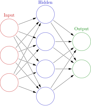
Why should a clinician care about the internals at all? Because understanding how these models learn is what lets you judge a paper’s claims: whether the authors guarded against memorising their data, whether they used enough examples, and whether the reported performance is likely to hold up in your own hospital. The diagram below shows the basic flow — raw inputs enter on the left, pass through hidden layers that build up more useful features, and emerge as a prediction on the right.

Figure 14.1: How a feedforward neural network is organised. Information flows from the **input layer** (one node per measurement — e.g. age, creatinine, blood pressure), through one or more **hidden layers** that combine those inputs into progressively more useful features, to an **output layer** that produces the prediction (here, a risk probability). Every node connects to every node in the next layer, and each connection carries a weight the network learns during training; a “deep” network simply has more hidden layers. Figure by Glosser.ca via Wikimedia Commons, licensed under CC BY-SA 3.0.

14.2.1 The Building Blocks

Neurons (nodes): Each neuron computes a weighted sum of its inputs, adds a bias, and applies a non-linear function (called an activation function):

\[a = f\left(\sum_{i=1}^{n} w_i x_i + b\right)\]

where $x_i$ are the inputs, $w_i$ are the weights, $b$ is the bias, and $f$ is the activation function. In clinical terms, this is exactly the structure of a risk score: each input (say, age, creatinine, blood pressure) is multiplied by a weight that says how much it matters, the weighted contributions are added up, an intercept (the bias $b$) is added, and the total is squashed into a usable range by $f$. A single neuron with a sigmoid activation is a logistic regression. The power of a network comes from wiring thousands of these simple units together so the later ones can act on features the earlier ones discovered.

Layers: Neurons are organised into layers:

Input layer: receives the raw data (pixel values, lab values, word embeddings).
Hidden layers: intermediate layers that learn increasingly abstract features — “hidden” simply means they sit between the input and output and never face the outside world directly. A network with many hidden layers is called “deep” — hence “deep learning.”
Output layer: produces the final prediction (a probability, a class label, a continuous value).

Activation functions: These are the non-linear “shaping” steps that give neural networks their power. Each neuron’s weighted sum is passed through one of these functions before moving on. Without them, stacking many layers would be pointless — chaining straight lines together just gives you another straight line, so the network could never learn curved or interacting relationships. Common choices include:

ReLU (Rectified Linear Unit): $f(x) = \max(0, x)$. In plain terms, it passes positive values through unchanged and replaces any negative value with zero — a simple on/off gate. It is the default for hidden layers because it is simple, fast, and effective.
Sigmoid: $f(x) = \frac{1}{1+e^{-x}}$. Used in the output layer for binary classification. You already know this from logistic regression.
Softmax: Generalises sigmoid to multiple classes. Used in the output layer for multi-class classification.

14.2.2 Training: Gradient Descent and Backpropagation

Neural networks learn by adjusting their weights to minimise a loss function — a single number measuring how wrong the predictions are (smaller is better). The whole point of training is to nudge the weights until that number is as small as possible. The process works as follows:

Forward pass: Feed data through the network to produce a prediction.
Compute loss: Compare the prediction to the true label using a loss function (cross-entropy for classification, mean squared error for regression).
Backward pass (backpropagation): Work out how much each weight contributed to the error, so we know which way to adjust it. (“Backpropagation” means the error signal is traced backwards through the network, from output to input, using the chain rule of calculus.)
Update weights: Adjust each weight a little in the direction that reduces the loss, scaled by a learning rate $\eta$ (the size of each adjustment):

\[w \leftarrow w - \eta \frac{\partial \mathcal{L}}{\partial w}\]

Read the update rule in plain language. The gradient $\partial \mathcal{L}/\partial w$ is the slope of the error for one weight — it points in the direction that makes the predictions worse, so we step the opposite way (hence the minus sign). The learning rate $\eta$ sets how big each step is. A useful mental picture is walking downhill in fog: the gradient is the steepest direction underfoot, and $\eta$ is how big a stride you take before re-checking your footing. Taking these downhill steps repeatedly is what “gradient descent” means.

This whole cycle repeats over many epochs — one epoch is a single complete pass through all the training data, so 50 epochs means the model has seen every patient 50 times. The learning rate matters a great deal: too large, and the model overshoots and oscillates; too small, and it learns painfully slowly.

You Already Know This Pattern

Gradient descent is not unique to deep learning. It is the same optimisation strategy used in logistic regression and many other statistical models. The difference is scale: a logistic regression with 10 predictors has 11 parameters; a deep neural network may have millions.

14.2.3 Regularisation: Preventing Overfitting

Deep networks have enormous capacity and will happily memorise the training data if you let them. This memorisation is called overfitting: the model learns the quirks and noise of the patients it was trained on, rather than the general pattern, and then performs poorly on new patients. For a clinician, this is the single most important failure mode to watch for — a model that looks brilliant in the development paper but collapses when applied to your own patients has almost certainly overfit. The strategies for preventing this parallel what you learned in Chapter 6, but with some additions:

Dropout: During training, randomly “turn off” a fraction of neurons in each layer for each batch. This stops the network from leaning too heavily on any single neuron and forces it to learn more robust, redundant features — a bit like training a clinical team so that no single member is a point of failure. Typical dropout rates range from 0.2 to 0.5 (i.e. 20–50% of neurons switched off at a time).
Weight decay (L2 regularisation): Gently penalise large weights, exactly as in ridge regression, to keep the model from over-relying on any one input.
Early stopping: Watch performance on a held-out validation set during training and stop as soon as it starts getting worse — the point at which the model begins memorising rather than learning.
Data augmentation: Artificially expand the training set by applying small random changes (rotations, flips, crops, colour jitter). This is especially important in medical imaging, where labelled data is scarce.

14.3 Clinical Example: Neural Network for Readmission Prediction

To connect these concepts to what you already know, let us apply a simple neural network to the hospital readmission data from Chapter 13. This is not a scenario where deep learning is the right tool — gradient-boosted trees will likely perform as well or better on tabular data — but it illustrates the mechanics.

The example follows the standard train / validate / test workflow. We train the model on most of the data, use a validation slice to decide when to stop and how to tune, and keep a test set untouched until the very end to give an honest estimate of how the model will perform on new patients.

flowchart LR
  D["All patient data"] --> TR["Training set<br/>(fit the weights)"]
  D --> VA["Validation set<br/>(tune & early stopping)"]
  D --> TE["Test set<br/>(final, one-time check)"]
  TR --> M["Neural network"]
  M -->|"check each epoch"| VA
  VA -->|"adjust / stop"| M
  M -->|"report final performance"| TE

Figure 14.2: The train / validate / test loop. The model learns on the training data, is checked repeatedly on the validation data to tune settings and trigger early stopping, and is finally judged once on the held-out test data.

Code

library(tidyverse)   # ggplot2 / dplyr / tibble
library(keras3)

# Simulate readmission data (same structure as Chapter 8)
set.seed(42)
n <- 1000

readmit_data <- tibble(
  age = rnorm(n, 68, 12),
  length_of_stay = rpois(n, 5) + 1,
  num_comorbidities = rpois(n, 3),
  prior_admissions = rpois(n, 1),
  discharge_hgb = rnorm(n, 11, 2),
  discharge_creatinine = rlnorm(n, 0.2, 0.5),
  has_diabetes = rbinom(n, 1, 0.35),
  has_chf = rbinom(n, 1, 0.25)
)

readmit_prob <- plogis(
  -1.2 +
    0.05 * (readmit_data$age - 68) +
    0.7 * readmit_data$prior_admissions +
    0.25 * readmit_data$num_comorbidities +
    1.3 * readmit_data$has_chf -
    0.25 * (readmit_data$discharge_hgb - 11)
)
readmit_data$readmitted <- rbinom(n, 1, readmit_prob)

# Prepare data: scale features, split into train/test
x <- readmit_data %>%
  select(-readmitted) %>%
  as.matrix()
y <- readmit_data$readmitted

# Standardize
x_mean <- apply(x, 2, mean)
x_sd <- apply(x, 2, sd)
x_scaled <- scale(x, center = x_mean, scale = x_sd)

# Train/test split
set.seed(123)
train_idx <- sample(n, 800)
x_train <- x_scaled[train_idx, ]
x_test <- x_scaled[-train_idx, ]
y_train <- y[train_idx]
y_test <- y[-train_idx]

# Define a simple feedforward neural network
model <- keras_model_sequential(input_shape = ncol(x_train)) %>%
  layer_dense(units = 32, activation = "relu") %>%
  layer_dropout(rate = 0.3) %>%
  layer_dense(units = 16, activation = "relu") %>%
  layer_dropout(rate = 0.3) %>%
  layer_dense(units = 1, activation = "sigmoid")

model %>%
  compile(
    optimizer = optimizer_adam(learning_rate = 0.001),
    loss = "binary_crossentropy",
    metrics = "AUC"
  )

# Train with early stopping
history <- model %>%
  fit(
    x_train,
    y_train,
    epochs = 50,
    batch_size = 32,
    validation_split = 0.2,
    callbacks = list(
      callback_early_stopping(
        patience = 5,
        restore_best_weights = TRUE
      )
    ),
    verbose = 0
  )

# Evaluate on test set
results <- model %>% evaluate(x_test, y_test, verbose = 0)
cat("Test loss:", round(results[[1]], 3), "\n")
cat("Test AUC:", round(results[[2]], 3), "\n")

Code

import numpy as np
import keras
from keras import layers, models, callbacks
from sklearn.model_selection import train_test_split
from sklearn.preprocessing import StandardScaler

# Simulate readmission data (same structure as Chapter 8)
np.random.seed(42)
n = 1000

age = np.random.normal(68, 12, n)
length_of_stay = np.random.poisson(5, n) + 1
num_comorbidities = np.random.poisson(3, n)
prior_admissions = np.random.poisson(1, n)
discharge_hgb = np.random.normal(11, 2, n)
discharge_creatinine = np.random.lognormal(0.2, 0.5, n)
has_diabetes = np.random.binomial(1, 0.35, n)
has_chf = np.random.binomial(1, 0.25, n)

X = np.column_stack([age, length_of_stay, num_comorbidities,
                     prior_admissions, discharge_hgb,
                     discharge_creatinine, has_diabetes, has_chf])

prob = 1 / (1 + np.exp(-(-1.2 + 0.05 * (age - 68) +
                          0.7 * prior_admissions +
                          0.25 * num_comorbidities +
                          1.3 * has_chf -
                          0.25 * (discharge_hgb - 11))))
y = np.random.binomial(1, prob)

# Split and scale
X_train, X_test, y_train, y_test = train_test_split(
    X, y, test_size=0.2, stratify=y, random_state=123
)
scaler = StandardScaler()
X_train = scaler.fit_transform(X_train)
X_test = scaler.transform(X_test)

# Define a simple feedforward neural network
model = models.Sequential([
    layers.Dense(32, activation="relu", input_shape=(X_train.shape[1],)),
    layers.Dropout(0.3),
    layers.Dense(16, activation="relu"),
    layers.Dropout(0.3),
    layers.Dense(1, activation="sigmoid")
])

model.compile(
    optimizer=keras.optimizers.Adam(learning_rate=0.001),
    loss="binary_crossentropy",
    metrics=[keras.metrics.AUC(name="auc")]
)

# Train with early stopping
history = model.fit(
    X_train, y_train,
    epochs=50,
    batch_size=32,
    validation_split=0.2,
    callbacks=[
        callbacks.EarlyStopping(
            patience=5, restore_best_weights=True
        )
    ],
    verbose=0
)

loss, auc = model.evaluate(X_test, y_test, verbose=0)
print(f"Test loss: {loss:.3f}")
print(f"Test AUC:  {auc:.3f}")

What the code is doing. This walks through the full life-cycle of a neural network on tabular data, end to end. First we simulate 1,000 patients and a true readmission risk that depends on age, prior admissions, comorbidities, heart failure, and discharge haemoglobin — so we know the right answer and can judge the model. We then standardise every feature (subtract the mean, divide by the standard deviation) so that no variable dominates simply because it is measured on a larger scale, and split the data into training and held-out test sets. The architecture is a small stack: an input layer, two hidden layers (32 then 16 neurons) with ReLU activations and 30% dropout between them to curb overfitting, and a single sigmoid output that emits a readmission probability. compile chooses the optimiser (Adam), the loss (binary cross-entropy, the same quantity logistic regression minimises), and the metric to watch (AUC). fit trains for up to 50 epochs but, thanks to early stopping with patience = 5, halts once the validation AUC stops improving (for 5 epochs in a row) and rewinds to the best weights. The final two lines report the test-set loss and AUC. The AUC is the headline number: the probability that the model ranks a randomly chosen readmitted patient above a randomly chosen non-readmitted one. Expect something in the 0.65–0.75 range for data this noisy.

Compare This to Chapter 8

Run the XGBoost model from Chapter 13 on the same data and compare the AUC. You will likely find that XGBoost matches or exceeds the neural network — with less code, less tuning, and immediate access to variable importance. This is the norm for tabular clinical data.

14.4 Key Architectures for Clinical Research

You do not need to understand every layer and parameter to use deep learning effectively. But you do need to understand which architecture suits which data type and why.

14.4.1 Convolutional Neural Networks (CNNs): Learning from Images

CNNs learn spatial hierarchies of features from images. Early layers detect simple things like edges and textures; deeper layers combine these into complex patterns (tumour boundaries, retinal vessel structures, skin lesion shapes). This is roughly how a radiologist’s eye works too — first noticing local detail, then assembling it into a diagnosis.

Instead of connecting every neuron to every pixel, CNNs use convolutional filters. A convolution is simply a small window (say $3 \times 3$ pixels) that slides across the image looking for one local pattern — for example a horizontal edge — and lights up wherever it finds it. Because the same window is reused everywhere, the model can spot that pattern anywhere in the image without having to relearn it for each location. Stacking many such filters across many layers builds up a rich hierarchy of features, from edges to whole anatomical structures.

Landmark clinical applications:

Application	Key Study	Architecture	Performance
Chest X-ray diagnosis	Rajpurkar et al. (2017)	DenseNet-121	Radiologist-level pneumonia detection
Diabetic retinopathy	Gulshan et al., JAMA 2016	Inception-v3	AUC 0.991 for referable DR
Skin cancer classification	Esteva et al., Nature 2017	Inception-v3	Dermatologist-level performance
Pathology	Campanella et al., Nature Medicine 2019	ResNet	Weakly supervised cancer detection in whole-slide images

From CNNs to Vision Transformers

Classic CNN architectures (ResNet, DenseNet) dominated medical imaging from 2015 to 2021. Since then, Vision Transformers (ViTs) have emerged as strong alternatives in research. ViTs split images into patches, treat each patch as a “token” (analogous to a word in NLP), and use self-attention to model relationships between patches. However, there is an “architectural gap” between research and clinical deployment: as of early 2026, nearly all FDA-cleared radiology AI devices still use CNNs, not transformers or foundation models (Lancet Digital Health, 2026). In the research literature, CNNs and ViTs achieve comparable performance on many tasks, and hybrid architectures are increasingly common.

14.4.2 Recurrent Networks and Transformers: Learning from Sequences

Recurrent Neural Networks (RNNs) were designed for sequential data — time series, text, and any data where order matters. The network reads the sequence one step at a time and carries along a running summary of what it has seen so far, called the hidden state (think of it as the network’s short-term memory). This lets it use information from earlier in the sequence when interpreting later steps.

Long Short-Term Memory (LSTM) networks solve the tendency of standard RNNs to forget things that happened long ago in the sequence. They use small “gates” — learned switches that decide what to keep, what to discard, and what to pass on at each step. LSTMs were the dominant architecture for clinical time series from roughly 2015 to 2022.

Transformers have largely superseded RNNs and LSTMs. Instead of reading a sequence one element at a time, transformers use self-attention — a mechanism that lets every element look at, and weigh the importance of, every other element at once. For a clinical note, this means the model can directly link “shortness of breath” early in the text to “heart failure” much later. Because all the comparisons happen simultaneously rather than step by step, transformers train faster and capture long-range relationships more effectively. Medformer (NeurIPS 2024) is the current state-of-the-art transformer architecture specifically designed for medical time series classification.

Clinical applications of sequential architectures:

Data Type	Example	Current Preferred Architecture
ECG tracings	Arrhythmia detection, digital biomarkers	Transformers
EEG signals	Seizure detection, ICU monitoring	Transformers with attention-based interpretability
ICU vital signs	Mortality prediction, clinical deterioration	Transformers, temporal CNNs
Wearable sensor data	Activity recognition, gait analysis	Temporal CNNs, hybrid models

14.4.3 Large Language Models: Learning from Clinical Text

The transformer architecture is also the foundation of large language models (LLMs). In clinical research, LLMs and their smaller predecessors have been applied to:

Named entity recognition: Automatically tagging the diseases, medications, procedures, and lab values mentioned in free-text clinical notes. Models like ClinicalBERT and PubMedBERT (~110M parameters) remain workhorses for this kind of structured extraction.
Information extraction: Pulling structured data from pathology and radiology reports.
Report generation: Drafting radiology or pathology reports from imaging studies.
Clinical question answering: Med-PaLM 2 achieved 86.5% on MedQA; Med-Gemini reached 91.1%. The MedHELM benchmark (Nature Medicine, 2025) tested 9 frontier LLMs across 121 medical tasks, finding scores of 0.73–0.85 for clinical note generation but only 0.56–0.72 for clinical decision support.

LLMs Are Not Clinical Decision-Making Tools (Yet)

LLMs can hallucinate — confidently generating plausible-sounding but factually wrong medical information (a fabricated drug interaction, a non-existent reference). They lack the ability to reason causally about individual patients. Current evidence supports their use as assistants (drafting notes, extracting structured data, literature search) rather than as autonomous clinical decision-makers. Always verify LLM outputs against primary sources.

14.4.4 Deep Learning for Survival Analysis

If you worked through Chapter 7, you know that time-to-event data requires special handling. Deep learning has extended survival analysis beyond the Cox model:

Model	Approach	Key Feature
DeepSurv (Katzman et al. 2018)	Neural network within Cox PH framework	Learns non-linear risk functions
DeepHit (Lee et al. 2018)	Custom loss; no parametric assumptions	Handles competing risks directly
SurvTRACE (2024)	Transformer-based	Models competing events with attention
DySurv (JAMIA, 2025)	Conditional variational autoencoder	Dynamic risk from longitudinal EHR data

For most clinical survival analysis, Cox regression and random survival forests remain the appropriate starting point. Deep survival models become relevant with high-dimensional inputs (imaging, genomics) or complex temporal patterns.

14.5 Transfer Learning and Foundation Models

Transfer learning is the single most important practical technique in deep learning for health research, and it is why deep learning is now feasible for groups with only modest datasets. The idea is simple: take a model that has already learned useful general features from a huge dataset, and adapt it to your specific task with a much smaller one. The clinical analogy is a trained radiologist who already knows how to read images in general — you only need to teach them the specifics of your new task, not how to see from scratch.

14.5.1 How Transfer Learning Works

Start with a pretrained model: A CNN trained on ImageNet (14 million natural images) has learned to detect edges, textures, shapes, and objects. These features transfer surprisingly well to medical images.
Replace the output layer: Swap the final classification head with one that predicts your clinical outcome.
Fine-tune: Train the modified model on your clinical dataset. You can freeze the pretrained layers (fast, works with very small datasets) or fine-tune all layers with a small learning rate (better performance, requires more data).

14.5.2 Foundation Models in Medicine

The field is moving beyond ImageNet toward domain-specific foundation models pretrained on medical data. A few open-source examples are listed below:

Model	Domain	Training Data	Published
MedSAM	Image segmentation	1.57M image-mask pairs, 10 modalities	Nature Communications, 2024
BiomedCLIP	Vision-language	15M biomedical image-text pairs	Microsoft, 2023
RETFound	Ophthalmology	1.6M retinal images, self-supervised	Nature, 2023
UNI	Pathology	100K+ whole-slide images	Nature Medicine, 2024
Virchow	Pathology	1.5M whole-slide images	Paige/Microsoft, 2024
Ark+	Chest Radiography	0.7M images	Nature, 2025
MedGemma 1.5	Multimodal (text, image)	>30M image-text pairs + text- and image-only datasets	Google, 2026

Practical Advice for Clinical Researchers

If you want to apply deep learning to medical images, do not train from scratch. Start with one or a few pretrained foundation models, and if needed and if you have computational capacity, fine-tune on your labelled data. With even a few hundred annotated images, you can achieve strong performance. This is the practical path for most clinical research groups.

14.5.3 Transfer Learning in Practice

The following example shows the complete workflow for fine-tuning a pretrained ResNet50 for binary image classification. In practice, you would replace the data loading step with your own clinical images.

Code

library(keras3)

# Load pretrained ResNet50 (trained on ImageNet, without classification head)
base_model <- application_resnet50(
  weights = "imagenet",
  include_top = FALSE,
  input_shape = c(224, 224, 3)
)
freeze_weights(base_model)

# Add new classification head for binary outcome
model <- keras_model_sequential(input_shape = c(224, 224, 3)) %>%
  base_model() %>%
  layer_global_average_pooling_2d() %>%
  layer_dropout(rate = 0.3) %>%
  layer_dense(units = 1, activation = "sigmoid")

model %>%
  compile(
    optimizer = optimizer_adam(learning_rate = 1e-4),
    loss = "binary_crossentropy",
    metrics = "AUC"
  )

# Data augmentation (rotation, flipping, shifting)
train_datagen <- image_data_generator(
  rescale = 1 / 255,
  rotation_range = 20,
  horizontal_flip = TRUE,
  validation_split = 0.2
)

# Point to your image directory organized as: images/class_0/ and images/class_1/
train_gen <- flow_images_from_directory(
  "path/to/images/",
  train_datagen,
  target_size = c(224, 224),
  batch_size = 32,
  class_mode = "binary",
  subset = "training"
)

val_gen <- flow_images_from_directory(
  "path/to/images/",
  train_datagen,
  target_size = c(224, 224),
  batch_size = 32,
  class_mode = "binary",
  subset = "validation"
)

# Fine-tune with early stopping
history <- model %>%
  fit(
    train_gen,
    epochs = 20,
    validation_data = val_gen,
    callbacks = list(
      callback_early_stopping(
        patience = 3,
        restore_best_weights = TRUE
      )
    )
  )

Code

import keras
from keras.applications import ResNet50
from keras import layers, models, callbacks

# Load pretrained ResNet50 (trained on ImageNet, without classification head)
base_model = ResNet50(weights="imagenet", include_top=False,
                      input_shape=(224, 224, 3))
base_model.trainable = False

# Data augmentation (rotation, flipping) applied inside the model
data_augmentation = models.Sequential([
    layers.RandomFlip("horizontal"),
    layers.RandomRotation(0.05),
])

# Add augmentation + new classification head for binary outcome
model = models.Sequential([
    layers.Rescaling(1.0 / 255),
    data_augmentation,
    base_model,
    layers.GlobalAveragePooling2D(),
    layers.Dropout(0.3),
    layers.Dense(1, activation="sigmoid")
])

model.compile(optimizer=keras.optimizers.Adam(learning_rate=1e-4),
              loss="binary_crossentropy",
              metrics=[keras.metrics.AUC(name="auc")])

# Point to your image directory organized as: images/class_0/ and images/class_1/
train_ds = keras.utils.image_dataset_from_directory(
    "path/to/images/", image_size=(224, 224),
    batch_size=32, validation_split=0.2,
    subset="training", seed=42
)

val_ds = keras.utils.image_dataset_from_directory(
    "path/to/images/", image_size=(224, 224),
    batch_size=32, validation_split=0.2,
    subset="validation", seed=42
)

# Fine-tune with early stopping
history = model.fit(
    train_ds, epochs=20, validation_data=val_ds,
    callbacks=[
        callbacks.EarlyStopping(
            patience=3, restore_best_weights=True
        )
    ]
)

What the code is doing. This is the workhorse recipe for medical imaging in a typical research group. Rather than training a network from scratch (which would need tens of thousands of labelled images), we load ResNet50 with its ImageNet weights already in place — a model that has already learned to detect edges, textures, and shapes from 14 million natural photographs. We discard its original 1,000-category classifier (include_top = FALSE) and freeze its weights so they are not disturbed. We then bolt on a fresh head — a pooling layer, dropout, and a single sigmoid neuron — which is the only part that learns from our clinical images. The augmentation layers (RandomFlip, RandomRotation) perform data augmentation: each epoch they show the network slightly rotated and flipped versions of the same images, artificially enlarging a small dataset and teaching the model to ignore irrelevant orientation. The image_dataset_from_directory call expects your images sorted into one folder per class. The practical takeaway is the pattern — freeze a pretrained backbone, train a small new head, augment aggressively — which lets you reach strong performance with only a few hundred annotated scans.

14.6 Practical Considerations

14.6.1 When to Use (and Not Use) Deep Learning

Scenario	Recommendation
Tabular EHR data, <50 features	Logistic regression or XGBoost
Tabular data combined with images or text	DL for the unstructured component; consider multimodal fusion
Medical images (X-ray, CT, MRI, pathology)	DL with transfer learning
Clinical notes, radiology reports	Transformer-based models
ECG, EEG, ICU time series	DL is appropriate; consider transformers or temporal CNNs
Survival analysis, standard covariates	Cox regression or random survival forests first

14.6.2 Data Requirements

Approach	Typical Data Needed
Training from scratch	Tens of thousands of labelled examples
Transfer learning (fine-tuning)	Hundreds to low thousands
Foundation model adaptation	As few as 50–100 examples for simple tasks
Self-supervised pretraining	Large amounts of unlabelled data

14.6.3 Compute

Approach	Hardware
Fine-tuning a pretrained model	Single GPU; Google Colab (free) works
Training a moderate model from scratch	1–4 GPUs; cloud instance ~$2–4/hour
Training a foundation model	GPU cluster; not realistic for most research groups
Running inference	CPU is often sufficient

14.6.4 Reporting Deep Learning Studies

If you publish research involving deep learning, several reporting guidelines apply:

TRIPOD+AI (Collins et al., BMJ 2024): 27-item checklist for prediction models using regression or ML. Applies to all prediction model studies.
CLAIM (Mongan, Moy, and Kahn, Radiology: AI 2020): Checklist for AI in Medical Imaging. Covers study design, data, model, evaluation, and discussion.
CONSORT-AI / SPIRIT-AI (Liu et al. and Rivera et al., Nature Medicine 2020): Extensions for reporting randomised trials and protocols involving AI.
MINIMAR (Hernandez-Boussard et al., JAMIA 2020): Minimum information for medical AI reporting.

14.6.5 Regulatory Context

As of early 2026, the FDA has authorised over 1,350 AI-enabled medical devices, with 76% in radiology. Nearly all are Class II devices cleared via the 510(k) pathway. The EU AI Act, which entered into force in August 2024, classifies AI-enabled medical devices as high-risk, with full compliance obligations from August 2026. If you are developing a model intended for clinical deployment, regulatory awareness is essential from the outset.

14.7 Challenges and Limitations

The External Validation Problem

A systematic review of 86 deep learning algorithms in radiology found that 81% exhibited decreased accuracy on external datasets, with nearly a quarter experiencing a substantial drop of 0.10 or greater in AUC. Domain shift — differences in patient demographics, imaging equipment, acquisition protocols, and disease prevalence between development and deployment sites — remains the greatest obstacle to clinical translation.

Fairness and bias: A 2024 study in Nature Medicine demonstrated that even if a model is optimised for fairness at a single site, fairness does not transfer to out-of-distribution datasets. Subgroup analysis across age, sex, and ethnicity is essential.

Interpretability: A systematic review of 67 studies (2019–2024) found that the addition of explainability methods (Grad-CAM, saliency maps) provided no statistically significant improvement in diagnostic accuracy beyond the AI prediction itself. Interpretability tools are valuable for debugging and trust-building, but they are not a substitute for rigorous external validation.

Temporal degradation: Clinical AI models can degrade over time as clinical practice, coding conventions, and patient populations change. Post-deployment monitoring is essential but rarely implemented.

14.8 Exercises

Exercise 1: Neural Network vs XGBoost on Tabular Data

Using the readmission dataset from this chapter, fit both a neural network and an XGBoost model. Compare their performance using 5-fold cross-validated AUC.

Code

library(tidyverse) # tibble()
library(keras3)
library(tidymodels)
library(xgboost)

# Use the readmit_data from above (or re-simulate it)
set.seed(42)
n <- 1000

readmit_data <- tibble(
  age = rnorm(n, 68, 12),
  length_of_stay = rpois(n, 5) + 1,
  num_comorbidities = rpois(n, 3),
  prior_admissions = rpois(n, 1),
  discharge_hgb = rnorm(n, 11, 2),
  discharge_creatinine = rlnorm(n, 0.2, 0.5),
  has_diabetes = rbinom(n, 1, 0.35),
  has_chf = rbinom(n, 1, 0.25)
)

readmit_prob <- plogis(
  -1.2 +
    0.05 * (readmit_data$age - 68) +
    0.7 * readmit_data$prior_admissions +
    0.25 * readmit_data$num_comorbidities +
    1.3 * readmit_data$has_chf -
    0.25 * (readmit_data$discharge_hgb - 11)
)
readmit_data$readmitted <- factor(
  rbinom(n, 1, readmit_prob),
  labels = c("No", "Yes")
)

# Your code:
# 1. Set up a tidymodels XGBoost workflow with 5-fold CV
# 2. Train a Keras neural network with 5-fold CV (use a loop over folds)
# 3. Compare AUC from both approaches
# 4. Which model performs better? Does this surprise you?

Code

import numpy as np
from sklearn.model_selection import StratifiedKFold, cross_val_score
from sklearn.preprocessing import StandardScaler
from sklearn.pipeline import make_pipeline
import xgboost as xgb
import keras
from keras import layers, models, callbacks
from sklearn.metrics import roc_auc_score

np.random.seed(42)
n = 1000

# Re-simulate readmission data (same as above)
# Your code:
# 1. Run 5-fold CV with XGBClassifier using cross_val_score
# 2. Run 5-fold CV with a Keras model (manual loop)
# 3. Compare mean AUC across folds
# 4. Which model performs better? Does this surprise you?

Solution

Code

# =============================================================================
# Chapter 8b, Exercise 1: Neural Network vs XGBoost on Tabular Data
# Fit both a neural network and XGBoost on the readmission dataset.
# Compare 5-fold cross-validated AUC.
# =============================================================================

library(tidyverse)
library(tidymodels)
library(keras3)

# --- Simulate readmission data (same as chapter) ---
set.seed(42)
n <- 1000

readmit_data <- tibble(
  age = rnorm(n, 68, 12),
  length_of_stay = rpois(n, 5) + 1,
  num_comorbidities = rpois(n, 3),
  prior_admissions = rpois(n, 1),
  discharge_hgb = rnorm(n, 11, 2),
  discharge_creatinine = rlnorm(n, 0.2, 0.5),
  has_diabetes = rbinom(n, 1, 0.35),
  has_chf = rbinom(n, 1, 0.25)
)

readmit_prob <- plogis(-3 + 0.02 * (readmit_data$age - 68) +
                         0.15 * readmit_data$prior_admissions +
                         0.1 * readmit_data$num_comorbidities +
                         0.3 * readmit_data$has_chf -
                         0.1 * readmit_data$discharge_hgb)
readmit_data$readmitted <- factor(rbinom(n, 1, readmit_prob),
                                   labels = c("No", "Yes"))

cat("Readmission rate:", mean(readmit_data$readmitted == "Yes"), "\n")

# --- XGBoost with 5-fold CV (using tidymodels) ---
set.seed(42)
folds <- vfold_cv(readmit_data, v = 5, strata = readmitted)

xgb_spec <- boost_tree(trees = 500, tree_depth = 4, learn_rate = 0.05,
                        min_n = 10) %>%
  set_engine("xgboost") %>%
  set_mode("classification")

xgb_wf <- workflow() %>%
  add_model(xgb_spec) %>%
  add_recipe(recipe(readmitted ~ ., data = readmit_data))

xgb_res <- fit_resamples(xgb_wf, resamples = folds,
                         metrics = metric_set(roc_auc))

xgb_metrics <- collect_metrics(xgb_res)
cat("\nXGBoost CV AUC:", xgb_metrics$mean, "+/-", xgb_metrics$std_err, "\n")

# --- Neural Network with 5-fold CV (manual loop) ---
x_all <- readmit_data %>% select(-readmitted) %>% as.matrix()
y_all <- as.numeric(readmit_data$readmitted == "Yes")

# Standardize features
x_mean <- apply(x_all, 2, mean)
x_sd   <- apply(x_all, 2, sd)
x_scaled <- scale(x_all, center = x_mean, scale = x_sd)

set.seed(42)
fold_ids <- vfold_cv(readmit_data, v = 5, strata = readmitted)
nn_aucs <- numeric(5)

for (i in seq_len(5)) {
  # Get train/validation indices
  train_idx <- fold_ids$splits[[i]] %>% analysis() %>% rownames() %>% as.integer()
  val_idx   <- fold_ids$splits[[i]] %>% assessment() %>% rownames() %>% as.integer()

  x_train <- x_scaled[train_idx, ]
  y_train <- y_all[train_idx]
  x_val   <- x_scaled[val_idx, ]
  y_val   <- y_all[val_idx]

  # Build neural network
  model <- keras_model_sequential(input_shape = ncol(x_train)) %>%
    layer_dense(units = 32, activation = "relu") %>%
    layer_dropout(rate = 0.3) %>%
    layer_dense(units = 16, activation = "relu") %>%
    layer_dropout(rate = 0.3) %>%
    layer_dense(units = 1, activation = "sigmoid")

  model %>% compile(
    optimizer = optimizer_adam(learning_rate = 0.001),
    loss = "binary_crossentropy",
    metrics = "AUC"
  )

  # Train with early stopping
  history <- model %>% fit(
    x_train, y_train,
    epochs = 50,
    batch_size = 32,
    validation_data = list(x_val, y_val),
    callbacks = list(
      callback_early_stopping(patience = 5, restore_best_weights = TRUE)
    ),
    verbose = 0
  )

  # Evaluate
  results <- model %>% evaluate(x_val, y_val, verbose = 0)
  nn_aucs[i] <- results[[2]]  # AUC metric
  cat(sprintf("  Fold %d: NN AUC = %.3f\n", i, nn_aucs[i]))
}

cat("\nNeural Network CV AUC:", mean(nn_aucs), "+/-", sd(nn_aucs) / sqrt(5), "\n")

# --- Comparison ---
cat("\n=== Comparison ===\n")
cat("XGBoost CV AUC:        ", round(xgb_metrics$mean, 3), "\n")
cat("Neural Network CV AUC: ", round(mean(nn_aucs), 3), "\n")

cat("\nInterpretation:\n")
cat("XGBoost typically matches or outperforms neural networks on tabular\n")
cat("clinical data. This is expected -- the Grinsztajn et al. (2022)\n")
cat("NeurIPS benchmark showed that tree-based models consistently\n")
cat("outperform neural networks on typical tabular datasets. Deep learning\n")
cat("excels on images, text, and sequences, not spreadsheets.\n")

Code

# =============================================================================
# Chapter 8b, Exercise 1: Neural Network vs XGBoost on Tabular Data
# Fit both a neural network and XGBoost on the readmission dataset.
# Compare 5-fold cross-validated AUC.
# =============================================================================

import numpy as np
import pandas as pd
from sklearn.model_selection import StratifiedKFold, cross_val_score
from sklearn.preprocessing import StandardScaler
from sklearn.metrics import roc_auc_score
import xgboost as xgb
import keras
from keras import layers, models, callbacks

# --- Simulate readmission data (same as chapter) ---
np.random.seed(42)
n = 1000

age = np.random.normal(68, 12, n)
length_of_stay = np.random.poisson(5, n) + 1
num_comorbidities = np.random.poisson(3, n)
prior_admissions = np.random.poisson(1, n)
discharge_hgb = np.random.normal(11, 2, n)
discharge_creatinine = np.random.lognormal(0.2, 0.5, n)
has_diabetes = np.random.binomial(1, 0.35, n)
has_chf = np.random.binomial(1, 0.25, n)

X = np.column_stack([age, length_of_stay, num_comorbidities,
                     prior_admissions, discharge_hgb,
                     discharge_creatinine, has_diabetes, has_chf])

# Generate outcome with known logistic relationship
prob = 1 / (1 + np.exp(-(-3 + 0.02 * (age - 68) +
                          0.15 * prior_admissions +
                          0.1 * num_comorbidities +
                          0.3 * has_chf -
                          0.1 * discharge_hgb)))
y = np.random.binomial(1, prob)
print(f"Readmission rate: {y.mean():.3f}")

# --- XGBoost with 5-fold CV ---
cv = StratifiedKFold(n_splits=5, shuffle=True, random_state=42)

xgb_model = xgb.XGBClassifier(
    n_estimators=500, learning_rate=0.05, max_depth=4,
    subsample=0.8, colsample_bytree=0.8,
    random_state=42, use_label_encoder=False, eval_metric='logloss'
)

xgb_scores = cross_val_score(xgb_model, X, y, cv=cv, scoring='roc_auc')
print(f"\nXGBoost CV AUC: {xgb_scores.mean():.3f} (+/- {xgb_scores.std():.3f})")

# --- Neural Network with 5-fold CV (manual loop) ---
nn_aucs = []
fold_idx = 0

for train_idx, val_idx in cv.split(X, y):
    fold_idx += 1

    # Split and scale
    scaler = StandardScaler()
    X_train = scaler.fit_transform(X[train_idx])
    X_val = scaler.transform(X[val_idx])
    y_train = y[train_idx]
    y_val = y[val_idx]

    # Build neural network (same architecture as chapter)
    keras.utils.set_random_seed(42)
    model = models.Sequential([
        layers.Dense(32, activation="relu", input_shape=(X_train.shape[1],)),
        layers.Dropout(0.3),
        layers.Dense(16, activation="relu"),
        layers.Dropout(0.3),
        layers.Dense(1, activation="sigmoid")
    ])

    model.compile(
        optimizer=keras.optimizers.Adam(learning_rate=0.001),
        loss="binary_crossentropy",
        metrics=[keras.metrics.AUC(name="auc")]
    )

    # Train with early stopping
    history = model.fit(
        X_train, y_train,
        epochs=50,
        batch_size=32,
        validation_data=(X_val, y_val),
        callbacks=[
            callbacks.EarlyStopping(patience=5, restore_best_weights=True)
        ],
        verbose=0
    )

    # Evaluate
    y_pred_prob = model.predict(X_val, verbose=0).ravel()
    fold_auc = roc_auc_score(y_val, y_pred_prob)
    nn_aucs.append(fold_auc)
    print(f"  Fold {fold_idx}: NN AUC = {fold_auc:.3f}")

nn_mean_auc = np.mean(nn_aucs)
nn_std_auc = np.std(nn_aucs)
print(f"\nNeural Network CV AUC: {nn_mean_auc:.3f} (+/- {nn_std_auc:.3f})")

# --- Comparison ---
print(f"\n=== Comparison ===")
print(f"XGBoost CV AUC:        {xgb_scores.mean():.3f}")
print(f"Neural Network CV AUC: {nn_mean_auc:.3f}")

print("\nInterpretation:")
print("XGBoost typically matches or outperforms neural networks on tabular")
print("clinical data. This is expected -- the Grinsztajn et al. (2022)")
print("NeurIPS benchmark showed that tree-based models consistently")
print("outperform neural networks on typical tabular datasets. Deep learning")
print("excels on images, text, and sequences, not spreadsheets.")

Exercise 2: Architecture Matching

For each of the following clinical tasks, identify (a) the most appropriate deep learning architecture, (b) whether deep learning is likely to outperform gradient-boosted trees, and (c) the most relevant reporting guideline. Write 2–3 sentences justifying each answer.

Predicting 30-day mortality from 15 structured EHR variables (age, labs, vitals, comorbidities).
Classifying skin lesions as benign or malignant from dermoscopy images.
Detecting atrial fibrillation from 12-lead ECG tracings.
Extracting medication names from unstructured discharge summaries.
Predicting length of stay from a combination of structured EHR data and a chest X-ray at admission.

Solution

Code

# =============================================================================
# Chapter 8b, Exercise 2: Architecture Matching
# For each clinical task, identify the best DL architecture, whether DL
# is likely to outperform gradient-boosted trees, and the reporting guideline.
# =============================================================================

# =============================================================================
# Task 1: Predicting 30-day mortality from 15 structured EHR variables
# =============================================================================
#
# (a) Architecture: Feedforward neural network (multi-layer perceptron) or,
#     better yet, gradient-boosted trees (XGBoost/LightGBM). With only 15
#     structured variables, a simple architecture suffices.
#
# (b) DL likely to outperform GBT? NO. This is classic tabular data with a
#     modest number of features. The Grinsztajn et al. (2022) NeurIPS
#     benchmark and subsequent clinical benchmarks consistently show that
#     tree-based models match or outperform neural networks on tabular data.
#     Logistic regression or XGBoost is the appropriate starting point.
#
# (c) Reporting guideline: TRIPOD+AI (Collins et al., BMJ 2024). This is a
#     standard clinical prediction model using structured data.

# =============================================================================
# Task 2: Classifying skin lesions as benign/malignant from dermoscopy images
# =============================================================================
#
# (a) Architecture: Convolutional Neural Network (CNN), specifically a
#     pretrained model like ResNet, EfficientNet, or Inception fine-tuned
#     on the dermoscopy images. A domain-specific foundation model could
#     also be used if available.
#
# (b) DL likely to outperform GBT? YES. Image data contains spatial
#     structure (edges, textures, shapes) that CNNs are specifically designed
#     to exploit. GBTs cannot process raw images and would require manual
#     feature extraction, which is inferior to learned CNN features. Esteva
#     et al. (Nature 2017) demonstrated dermatologist-level performance.
#
# (c) Reporting guideline: CLAIM (Checklist for AI in Medical Imaging,
#     Mongan et al., Radiology: AI 2020), supplemented by TRIPOD+AI.

# =============================================================================
# Task 3: Detecting atrial fibrillation from 12-lead ECG tracings
# =============================================================================
#
# (a) Architecture: Transformer-based model or temporal CNN. The chapter
#     notes that transformers are the current preferred architecture for ECG
#     data. Medformer (NeurIPS 2024) is specifically designed for medical
#     time series classification.
#
# (b) DL likely to outperform GBT? YES. ECG data is sequential with complex
#     temporal patterns. GBTs would require extensive manual feature
#     engineering (interval measurements, morphology features), whereas DL
#     can learn directly from the raw waveform. Hannun et al. (Nature
#     Medicine 2019) demonstrated cardiologist-level arrhythmia detection.
#
# (c) Reporting guideline: TRIPOD+AI for the prediction model, potentially
#     supplemented by CLAIM if imaging is involved (e.g., ECG images rather
#     than signal data).

# =============================================================================
# Task 4: Extracting medication names from unstructured discharge summaries
# =============================================================================
#
# (a) Architecture: Transformer-based language model, such as ClinicalBERT
#     or PubMedBERT for named entity recognition (NER). These pretrained
#     models understand medical vocabulary and can be fine-tuned for NER.
#
# (b) DL likely to outperform GBT? YES, decisively. This is a natural
#     language processing task. GBTs cannot process raw text meaningfully.
#     Transformer-based models understand context, synonyms, and medical
#     abbreviations. Rule-based and dictionary approaches are alternatives,
#     but modern NER with transformers is superior.
#
# (c) Reporting guideline: TRIPOD+AI. No specific imaging guideline applies.
#     MINIMAR (Hernandez-Boussard et al., JAMIA 2020) may also be relevant
#     as a minimum reporting standard.

# =============================================================================
# Task 5: Predicting length of stay from structured EHR + chest X-ray
# =============================================================================
#
# (a) Architecture: Multimodal fusion model. A CNN (e.g., pretrained
#     ResNet) processes the chest X-ray to extract image features. These
#     are concatenated with the structured EHR features and fed into a
#     combined prediction head (either a feedforward network or GBT on
#     the fused features).
#
# (b) DL likely to outperform GBT? PARTIALLY. The DL component is necessary
#     for the image. For the structured data alone, GBTs may be equal or
#     better. The optimal approach may be a hybrid: use a CNN to extract
#     image features, then combine those features with structured data in
#     a GBT. Recent work on multimodal fusion suggests this hybrid approach
#     can outperform either modality alone.
#
# (c) Reporting guideline: TRIPOD+AI for the overall prediction model,
#     supplemented by CLAIM for the imaging component. Both should be
#     addressed since the model involves medical imaging.

cat("This exercise is conceptual. See the comments in this file for the\n")
cat("complete answers to all five clinical tasks.\n")

Code

# =============================================================================
# Chapter 8b, Exercise 2: Architecture Matching
# For each clinical task, identify the best DL architecture, whether DL
# is likely to outperform gradient-boosted trees, and the reporting guideline.
# =============================================================================

# =============================================================================
# Task 1: Predicting 30-day mortality from 15 structured EHR variables
# =============================================================================
#
# (a) Architecture: Feedforward neural network (MLP) or, better yet,
#     gradient-boosted trees (XGBoost/LightGBM). With only 15 structured
#     variables, a simple architecture suffices.
#
# (b) DL likely to outperform GBT? NO. This is classic tabular data with a
#     modest number of features. The Grinsztajn et al. (2022) NeurIPS
#     benchmark and subsequent clinical benchmarks consistently show that
#     tree-based models match or outperform neural networks on tabular data.
#
# (c) Reporting guideline: TRIPOD+AI (Collins et al., BMJ 2024). Standard
#     clinical prediction model using structured data.

# =============================================================================
# Task 2: Classifying skin lesions as benign/malignant from dermoscopy images
# =============================================================================
#
# (a) Architecture: CNN (e.g., pretrained ResNet, EfficientNet, or Inception
#     fine-tuned on dermoscopy images). A domain-specific foundation model
#     could also be used if available.
#
# (b) DL likely to outperform GBT? YES. Image data contains spatial
#     structure that CNNs exploit. GBTs cannot process raw images. Esteva
#     et al. (Nature 2017) demonstrated dermatologist-level performance.
#
# (c) Reporting guideline: CLAIM (Mongan et al., Radiology: AI 2020),
#     supplemented by TRIPOD+AI.

# =============================================================================
# Task 3: Detecting atrial fibrillation from 12-lead ECG tracings
# =============================================================================
#
# (a) Architecture: Transformer-based model or temporal CNN. Transformers
#     are the current preferred architecture for ECG data. Medformer
#     (NeurIPS 2024) is designed for medical time series classification.
#
# (b) DL likely to outperform GBT? YES. ECG data is sequential with complex
#     temporal patterns. DL can learn directly from raw waveforms, whereas
#     GBTs require extensive manual feature engineering.
#
# (c) Reporting guideline: TRIPOD+AI, potentially supplemented by CLAIM if
#     ECG images rather than signal data are used.

# =============================================================================
# Task 4: Extracting medication names from unstructured discharge summaries
# =============================================================================
#
# (a) Architecture: Transformer-based language model (ClinicalBERT or
#     PubMedBERT) for named entity recognition (NER). These models
#     understand medical vocabulary and context.
#
# (b) DL likely to outperform GBT? YES, decisively. This is an NLP task.
#     GBTs cannot process raw text meaningfully. Transformer-based NER
#     models understand context, synonyms, and medical abbreviations.
#
# (c) Reporting guideline: TRIPOD+AI. MINIMAR (Hernandez-Boussard et al.,
#     JAMIA 2020) also applicable as minimum reporting standard.

# =============================================================================
# Task 5: Predicting length of stay from structured EHR + chest X-ray
# =============================================================================
#
# (a) Architecture: Multimodal fusion model. A CNN (pretrained ResNet)
#     extracts image features from the chest X-ray. These are concatenated
#     with structured EHR features and fed into a combined prediction head.
#
# (b) DL likely to outperform GBT? PARTIALLY. DL is necessary for the image
#     component. For structured data alone, GBTs may be equal or better.
#     A hybrid approach (CNN for image features, then GBT on fused features)
#     may be optimal.
#
# (c) Reporting guideline: TRIPOD+AI for the prediction model, supplemented
#     by CLAIM for the imaging component.

print("This exercise is conceptual. See the comments in this file for the")
print("complete answers to all five clinical tasks.")

Exercise 3: Critical Appraisal of a Deep Learning Study

Find a recent (2024 or later) paper that applies deep learning to a clinical task in your area of interest. Evaluate it against the CLAIM or TRIPOD+AI checklist:

Was the model externally validated? If so, how did performance compare to internal validation?
Were subgroup analyses reported (by age, sex, ethnicity)?
Was the model compared to a simpler baseline (e.g., logistic regression)?
Were the training data, code, and model weights made available?
Based on your assessment, how close is this model to clinical deployment? What would you want to see before trusting it with patient care?

Solution

Code

# =============================================================================
# Chapter 8b, Exercise 3: Critical Appraisal of a Deep Learning Study
# Evaluate a DL paper against the CLAIM or TRIPOD+AI checklist.
# This is a conceptual/guided exercise -- the template below provides
# the framework for appraising any DL study.
# =============================================================================

# =============================================================================
# INSTRUCTIONS:
# Find a recent (2024 or later) paper applying deep learning to a clinical
# task in your area of interest. Use this template to evaluate it.
# =============================================================================

# =============================================================================
# Question 1: Was the model externally validated?
# =============================================================================
#
# Look for:
# - Was the model tested on data from a DIFFERENT institution, time period,
#   or geographic region than the training data?
# - If yes, how did external performance compare to internal (e.g., was there
#   a drop in AUC)?
#
# Example answer:
# "The model was validated on data from Hospital B after training on Hospital A.
#  Internal AUC was 0.92; external AUC dropped to 0.84 -- a 0.08 decrease.
#  This is consistent with the systematic review finding that 81% of DL models
#  show decreased accuracy on external datasets."
#
# Red flag: If NO external validation was performed, the results should be
# treated as preliminary. Internal CV alone is insufficient for clinical claims.

# =============================================================================
# Question 2: Were subgroup analyses reported?
# =============================================================================
#
# Look for:
# - Performance broken down by age, sex, race/ethnicity
# - Any mention of fairness or equity analysis
# - Performance in clinically important subgroups (e.g., patients with
#   comorbidities, different disease severity)
#
# Example answer:
# "The paper reported AUC by sex (male: 0.90, female: 0.87) but did not
#  report performance by race/ethnicity or age group. Given the known issue
#  of fairness non-transferability across sites (Nature Medicine 2024),
#  this is a significant omission."

# =============================================================================
# Question 3: Was the model compared to a simpler baseline?
# =============================================================================
#
# Look for:
# - Comparison against logistic regression, random forest, or XGBoost
# - If the DL model only marginally outperforms the baseline, the added
#   complexity may not be justified
#
# Example answer:
# "The paper compared DL (AUC 0.91) to logistic regression (AUC 0.85) and
#  random forest (AUC 0.88). The improvement over RF is modest (0.03),
#  raising questions about whether the DL model's added complexity and
#  reduced interpretability are justified."

# =============================================================================
# Question 4: Were training data, code, and model weights shared?
# =============================================================================
#
# Look for:
# - Public dataset or data sharing agreement
# - Code repository (GitHub, GitLab)
# - Pretrained model weights available for download
# - FAIR data principles
#
# Example answer:
# "Code was shared on GitHub. The training data is from a private hospital
#  system and is not publicly available, though the authors describe a
#  data sharing agreement. Model weights were not released."

# =============================================================================
# Question 5: How close is this model to clinical deployment?
# =============================================================================
#
# Consider:
# - Has it been externally validated across multiple sites?
# - Has it been tested prospectively (not just retrospectively)?
# - Has a clinical workflow been designed for how it would be used?
# - Has a regulatory pathway been identified (e.g., FDA 510(k), EU MDR)?
# - Has a monitoring plan for post-deployment performance been described?
# - What are the potential failure modes and harms?
#
# Example answer:
# "This model is at an early research stage. While the internal results are
#  promising, the model has been validated at only one external site with a
#  modest sample. Before clinical deployment, I would want to see:
#  (1) multi-site external validation,
#  (2) a prospective pilot study in clinical workflow,
#  (3) subgroup analysis across demographics,
#  (4) calibration assessment,
#  (5) a monitoring plan for detecting model drift over time."

cat("This exercise is a guided template for critical appraisal.\n")
cat("See the comments for the framework to evaluate any DL paper.\n")
cat("Students should find their own paper and fill in the answers.\n")

Code

# =============================================================================
# Chapter 8b, Exercise 3: Critical Appraisal of a Deep Learning Study
# Evaluate a DL paper against the CLAIM or TRIPOD+AI checklist.
# This is a conceptual/guided exercise -- the template below provides
# the framework for appraising any DL study.
# =============================================================================

# =============================================================================
# INSTRUCTIONS:
# Find a recent (2024 or later) paper applying deep learning to a clinical
# task in your area of interest. Use this template to evaluate it.
# =============================================================================

# =============================================================================
# Question 1: Was the model externally validated?
# =============================================================================
#
# Look for:
# - Was the model tested on data from a DIFFERENT institution, time period,
#   or geographic region than the training data?
# - If yes, how did external performance compare to internal (e.g., was there
#   a drop in AUC)?
#
# Example answer:
# "The model was validated on data from Hospital B after training on Hospital A.
#  Internal AUC was 0.92; external AUC dropped to 0.84 -- a 0.08 decrease.
#  This is consistent with the systematic review finding that 81% of DL models
#  show decreased accuracy on external datasets."
#
# Red flag: If NO external validation was performed, the results should be
# treated as preliminary.

# =============================================================================
# Question 2: Were subgroup analyses reported?
# =============================================================================
#
# Look for:
# - Performance broken down by age, sex, race/ethnicity
# - Any mention of fairness or equity analysis
# - Performance in clinically important subgroups
#
# Example answer:
# "The paper reported AUC by sex (male: 0.90, female: 0.87) but did not
#  report performance by race/ethnicity or age group. Given the known issue
#  of fairness non-transferability across sites, this is a significant
#  omission."

# =============================================================================
# Question 3: Was the model compared to a simpler baseline?
# =============================================================================
#
# Look for:
# - Comparison against logistic regression, random forest, or XGBoost
# - If the DL model only marginally outperforms the baseline, the added
#   complexity may not be justified
#
# Example answer:
# "The paper compared DL (AUC 0.91) to logistic regression (AUC 0.85) and
#  random forest (AUC 0.88). The improvement over RF is modest (0.03)."

# =============================================================================
# Question 4: Were training data, code, and model weights shared?
# =============================================================================
#
# Look for:
# - Public dataset or data sharing agreement
# - Code repository (GitHub, GitLab)
# - Pretrained model weights available
#
# Example answer:
# "Code was shared on GitHub. Training data is from a private hospital
#  system. Model weights were not released."

# =============================================================================
# Question 5: How close is this model to clinical deployment?
# =============================================================================
#
# Consider:
# - Has it been externally validated across multiple sites?
# - Has it been tested prospectively?
# - Has a clinical workflow been designed?
# - Has a regulatory pathway been identified?
# - Has a monitoring plan been described?
#
# Example answer:
# "This model is at an early research stage. Before clinical deployment,
#  I would want to see:
#  (1) multi-site external validation,
#  (2) a prospective pilot study,
#  (3) subgroup analysis across demographics,
#  (4) calibration assessment,
#  (5) a monitoring plan for model drift."

print("This exercise is a guided template for critical appraisal.")
print("See the comments for the framework to evaluate any DL paper.")
print("Students should find their own paper and fill in the answers.")

14.9 Summary

Concept	Key Takeaway
When to use deep learning	Images, text, time series, and sequences — not tabular data
Neural network basics	Weighted sums + non-linear activations, stacked in layers
CNNs	Learn spatial features from images via convolutional filters
Transformers	Use self-attention to model relationships in sequences; dominant for NLP and increasingly for imaging
LLMs in medicine	Strong for extraction and generation; not reliable for autonomous decision-making
Transfer learning	Start from pretrained weights; fine-tune on your data
Foundation models	Domain-specific pretrained models (MedSAM, RETFound, UNI) dramatically reduce data requirements
External validation	81% of radiology DL models degrade on external data
Reporting	Use TRIPOD+AI, CLAIM, CONSORT-AI, or MINIMAR as appropriate

14.10 References and Further Reading

For deep learning foundations, see Goodfellow et al. (2016), Zhang et al. (2023) (an interactive textbook, more practical than traditional textbooks), and Howard and Gugger (2020) (companion to the free fast.ai course).
For tabular data benchmarks, see Grinsztajn et al. (2022).
For clinical AI applications, see Ma et al. (2024) (foundation model for medical image analysis), Zhou et al. (2023) (foundation model for retinal image analysis), Bedi et al. (2025) (foundation model for medical language understanding), and Wiegrebe et al. (2024) (foundation model for survival analysis).
For reporting standards, see Collins et al. (2024) (TRIPOD+AI).

Bedi, Sujay, Helen Cui, Michael Fuentes, et al. 2025. “MedHELM: Holistic Evaluation of Large Language Models for Medical Tasks.” Nature Medicine. The most comprehensive LLM evaluation for clinical tasks, testing 9 frontier models across 121 tasks.

Collins, Gary S, Karel G M Moons, Paula Dhiman, et al. 2024. “TRIPOD+AI Statement: Updated Guidance for Reporting Clinical Prediction Models That Use Regression or Machine Learning Methods.” BMJ 385: e078378. https://doi.org/10.1136/bmj-2023-078378.

Goodfellow, Ian, Yoshua Bengio, and Aaron Courville. 2016. Deep Learning. MIT Press. https://www.deeplearningbook.org/. The definitive theoretical reference. Chapters 6 (deep feedforward networks), 9 (CNNs), and 10 (RNNs) are directly relevant.

Grinsztajn, Léo, Edouard Oyallon, and Gaël Varoquaux. 2022. “Why Do Tree-Based Models Still Outperform Deep Learning on Typical Tabular Data?” Advances in Neural Information Processing Systems (NeurIPS) 35. The benchmark study demonstrating that XGBoost consistently outperforms neural networks on tabular datasets. Essential reading before choosing deep learning for structured clinical data.

Howard, Jeremy, and Sylvain Gugger. 2020. Deep Learning for Coders with Fastai and PyTorch. O’Reilly Media. Companion to the free fast.ai course. Top-down, coding-first approach ideal for researchers who want to apply deep learning without years of theory.

Katzman, Jared L, Uri Shaham, Alexander Cloninger, Jonathan Bates, Tingting Jiang, and Yuval Kluger. 2018. “DeepSurv: Personalized Treatment Recommender System Using a Cox Proportional Hazards Deep Neural Network.” BMC Medical Research Methodology 18 (1): 24. https://doi.org/10.1186/s12874-018-0482-1. Replaces the linear predictor of a Cox model with a neural network, so non-linear and interacting risk relationships can be learned while keeping the proportional hazards framework.

Lee, Changhee, William R Zame, Jinsung Yoon, and Mihaela van der Schaar. 2018. “DeepHit: A Deep Learning Approach to Survival Analysis with Competing Risks.” Proceedings of the AAAI Conference on Artificial Intelligence 32: 2314–21. https://doi.org/10.1609/aaai.v32i1.11842. Models the discrete-time distribution of event times directly with a custom loss, avoiding proportional hazards assumptions and handling competing risks natively.

Ma, Jun, Yuting He, Feifei Li, Lin Han, Chenyu You, and Bo Wang. 2024. “Segment Anything in Medical Images.” Nature Communications 15: 654. https://doi.org/10.1038/s41467-024-44824-z. The MedSAM paper: a foundation model for universal medical image segmentation trained on 1.57 million image-mask pairs across 10 modalities.

Rajpurkar, Pranav, Jeremy Irvin, Kaylie Zhu, et al. 2017. CheXNet: Radiologist-Level Pneumonia Detection on Chest X-Rays with Deep Learning. https://doi.org/10.48550/arXiv.1711.05225. A 121-layer DenseNet trained on ChestX-ray14. Widely cited as a demonstration of radiologist-level performance on a single finding; note it remains a preprint.

Wiegrebe, Simon, Philipp Kopper, Bernd Bischl, and Andreas Bender. 2024. “Deep Learning for Survival Analysis: A Review.” Artificial Intelligence Review 57. https://doi.org/10.1007/s10462-023-10681-3. Comprehensive taxonomy covering DeepSurv, DeepHit, neural ODEs, and transformer-based approaches.

Zhang, Aston, Zachary C Lipton, Mu Li, and Alexander J Smola. 2023. Dive into Deep Learning. Cambridge University Press. https://d2l.ai/. An interactive textbook with executable code in PyTorch, TensorFlow, and JAX. More practical and accessible than Goodfellow et al. Adopted at over 500 universities.

Zhou, Yukun, Mark A Chia, Siegfried K Wagner, et al. 2023. “A Foundation Model for Generalizable Disease Detection from Retinal Images.” Nature 622: 156–63. https://doi.org/10.1038/s41586-023-06555-x. RETFound: self-supervised pretraining on 1.6 million retinal images, with strong downstream performance from minimal fine-tuning.