flowchart LR
    A[Research question] --> B[Search the literature]
    B --> C[Screen and select studies]
    C --> D[Appraise quality<br/>risk of bias]
    D --> E[Extract effect estimates]
    E --> F[Meta-analysis:<br/>pool into one estimate]
    F --> G[Forest plot,<br/>heterogeneity, bias checks]
24 Meta-Analysis for Evidence Synthesis
24.1 Introduction
A single study, no matter how well designed, provides only one piece of evidence. Meta-analysis is the statistical method for combining results from multiple independent studies addressing the same question, producing a more precise and more generalisable estimate of an effect.
As a health researcher you will meet meta-analyses constantly: they underpin clinical guidelines, they settle (and unsettle) treatment decisions, and they are often the papers your colleagues cite at you. Whether you are running one or reading one, what matters is understanding how the numbers get combined and what can go wrong — because when a meta-analysis is wrong, it is wrong with authority.
This chapter is deliberately narrow. It covers the core of an aggregate-data meta-analysis of a binary outcome, which is the overwhelming majority of what appears in clinical journals, and it covers it properly: how the pooling works, how to read a forest plot, how to think about heterogeneity, and how to detect the one failure mode that has misled clinical practice most often. Section 24.12 points you at the more specialised methods without pretending to teach them in a paragraph.
NoteSystematic review vs meta-analysis
A systematic review is the process of comprehensively searching for, selecting, and appraising studies. A meta-analysis is the statistical component — combining the numbers. You can have a systematic review without a meta-analysis (if the studies are too different to combine), but you should never have a meta-analysis without a systematic review.
The diagram below shows where the meta-analysis fits in the wider pipeline. Most of the work is finding and appraising studies; the statistical pooling is the final step.
24.2 What a Meta-Analysis Combines
Each study contributes an effect estimate — a single number summarising how big the effect was (“the drug cut the risk of stroke by 30%”) — and a measure of its precision, meaning how confident we are in that number (a standard error or confidence interval). The meta-analysis computes a weighted average: rather than treating every study equally, it gives more precise studies more say. This is inverse-variance weighting, because each study’s weight is one divided by its variance.
\[ \hat{\theta}_{\text{pooled}} = \frac{\sum_{i=1}^{k} w_i \hat{\theta}_i}{\sum_{i=1}^{k} w_i} \]
where \(\hat{\theta}_i\) is the effect estimate from study \(i\), \(w_i\) its weight, and \(k\) the number of studies. In plain terms: a large, precise trial pulls the combined answer towards its own result more strongly than a small, imprecise one — exactly as your intuition would suggest.
Hold on to that sentence. Almost everything that goes wrong in a meta-analysis is a disagreement about how much more say the big trials should get.
24.3 Effect Measures
The choice of effect measure depends on the type of outcome.
Binary outcomes (died / did not die, event / no event):
| Measure | Formula | When to use |
|---|---|---|
| Risk ratio (RR) | \(\frac{a/(a+b)}{c/(c+d)}\) | Cohort studies and trials; the most interpretable choice for clinicians |
| Odds ratio (OR) | \(\frac{ad}{bc}\) | Case-control studies; logistic regression |
| Risk difference (RD) | \(\frac{a}{a+b} - \frac{c}{c+d}\) | When the absolute risk is what matters for a decision |
Here \(a, b, c, d\) are the cells of a 2x2 table (treatment events, treatment non-events, control events, control non-events). Ratios are pooled on the log scale, because their sampling distributions are roughly normal there, and back-transformed for presentation.
Continuous outcomes:
| Measure | Formula | When to use |
|---|---|---|
| Mean difference (MD) | \(\bar{X}_T - \bar{X}_C\) | All studies use the same measurement scale |
| Standardised mean difference (SMD) | \(\dfrac{\bar{X}_T - \bar{X}_C}{S_{\text{pooled}}}\) | Studies use different scales for the same construct (e.g. different depression questionnaires) |
Here \(\bar{X}_T\) and \(\bar{X}_C\) are the average outcomes in the treatment and control groups. \(S_{\text{pooled}}\) is the pooled standard deviation: how much patients within a group differ from one another, combined across the two arms.
\[ S_{\text{pooled}} = \sqrt{\frac{(n_T - 1)\,S_T^2 + (n_C - 1)\,S_C^2}{n_T + n_C - 2}} \]
where \(n_T\) and \(n_C\) are the two group sizes and \(S_T\) and \(S_C\) the standard deviations within each group. It is essentially a sample-size-weighted average of those two standard deviations — not the standard deviation of the difference, and not the standard error.
Dividing by it is what makes different measurement scales comparable. Suppose one trial measured depression on a 0–63 questionnaire and improved scores by 6 points, while another used a 0–52 questionnaire and improved them by 4. Those raw numbers cannot be averaged together. But if patients within a group typically varied by 12 points on the first scale and 8 points on the second, then both trials moved patients by half of that typical variation, and the SMD is 0.5 in both. The SMD expresses the effect in units of how much patients differ from each other, so SMD = 0.5 means the average treated patient ended up half a standard deviation better off than the average control patient.
The cost is interpretability. “Half a standard deviation” is not a clinical quantity, and it depends on how variable the recruited population happened to be: a trial with narrow eligibility criteria has a small \(S_{\text{pooled}}\) and therefore reports a larger SMD for exactly the same real benefit. Use the plain mean difference whenever the studies share a scale.
The SMD is also known as Hedges’ g (with a small-sample correction applied, which is the version you should use) or Cohen’s d (without it).
WarningThe effect measure is not just a presentation choice
It changes which asymmetry tests are valid later (Section 24.10), and the odds ratio in particular has a mathematical quirk that makes the standard publication-bias test unreliable. Decide the measure from the clinical question, then pick methods that suit it — not the other way round.
24.4 The Running Example: Magnesium After a Heart Attack
Every analysis in this chapter uses one real dataset, so that the methods can be compared on identical evidence.
In the 1980s and early 1990s, a series of randomised trials tested whether giving intravenous magnesium to patients having an acute myocardial infarction reduced mortality. Magnesium is cheap, widely available, and biologically plausible as a cardioprotective agent. Sixteen trials accumulated. They are shipped with metafor as dat.egger2001, taken from Table 18.2 of Egger et al. (2001).
Code
library(metafor)   # for the dataset
library(tidyverse) # for the summary below

mag <- dat.egger2001 |>
  mutate(n_total = n1i + n2i)

# ai / n1i = deaths / patients on magnesium; ci / n2i = deaths / patients on control
mag |>
  transmute(trial = paste(study, year), magnesium = paste0(ai, "/", n1i),
            control = paste0(ci, "/", n2i), n_total) |>
  arrange(n_total) |>
  as.data.frame() |>
  print(row.names = FALSE)
trial magnesium control n_total
Bertschat 1989 0/22 1/21 43
Ceremuzynski 1989 1/25 3/23 48
Pereira 1990 1/27 7/27 54
Golf 1991 5/23 13/33 56
Morton 1984 1/40 2/36 76
Abraham 1987 1/48 1/46 94
Shechter 1989 1/59 9/56 115
Singh 1990 6/76 11/75 151
Shechter 1991 2/89 12/80 169
Shechter 1995 4/107 17/108 215
Thogersen 1991 4/130 8/122 252
Rasmussen 1986 9/135 23/135 270
Feldstedt 1988 10/150 8/148 298
Smith 1986 2/200 7/200 400
LIMIT-2 1992 90/1159 118/1157 2316
ISIS-4 1995 2216/29011 2103/29039 58050Look at the right-hand column before reading on. Thirteen of the sixteen trials randomised fewer than 400 patients in total; the largest randomised 58,050 and accounts for 93% of all the patients ever studied. That imbalance is the whole story of this chapter, and it is typical rather than exceptional: most clinical literatures consist of many small studies and one or two large ones.
We will build up the standard analysis, and only in Section 24.10 reveal what actually happened.
24.5 Fixed-Effect vs Random-Effects Models
The single most consequential choice in a meta-analysis is whether you assume the studies are all estimating one true effect or a range of true effects.
The next few pages use a handful of Greek symbols, so here is the whole vocabulary in one place. You can read the rest of the chapter with nothing more than this.
NoteThe symbols in this chapter, in words
| Symbol | Read it as | What it means here |
|---|---|---|
| \(\theta\) | “theta” | A true effect — the answer we would get from an infinitely large, perfect study. Greek letters are for quantities that exist but are never observed. |
| \(\hat{\theta}\) | “theta hat” | An estimate of that effect, calculated from data actually collected. The hat always means “our best guess at, from a sample”. |
| \(\theta_i\), \(\hat{\theta}_i\) | “theta i” | The true effect, and the estimate, in study number \(i\). The subscript just numbers the studies. |
| \(k\) | “k” | The number of studies being pooled (here, 16). |
| \(\hat{\sigma}_i^2\) | “sigma squared i” | Study \(i\)’s within-study variance: how much its own result would bounce around if that same trial were repeated. It is the square of the standard error, so a big trial has a small \(\hat{\sigma}_i^2\). |
| \(\tau^2\), \(\hat{\tau}^2\) | “tau squared” | The between-study variance: how much the true effects genuinely differ from one study to the next. |
| \(\mu\) | “mu” | The average of the true effects across studies — what a random-effects model is actually estimating. |
| \(w_i\) | “w i” | The weight given to study \(i\) when averaging. |
| \(\theta_i \sim N(\mu, \tau^2)\) | “theta i is normally distributed with mean mu and variance tau squared” | The true effects are scattered in a bell curve centred on \(\mu\), whose width is \(\tau\). |
Whenever a formula looks opaque, read the hats as “estimated”, the subscript \(i\) as “for this one study”, and \(\sigma\) and \(\tau\) as “noise within a study” and “real differences between studies”. Appendix B has a fuller list for the rest of the book.
The fixed-effect model assumes every study estimates the same true effect \(\theta\); differences between results are pure sampling noise, like getting slightly different averages each time you measure the same group of patients. Weights are the inverse of the within-study variance:
\[ w_i^{\text{FE}} = \frac{1}{\hat{\sigma}_i^2} \]
In words: a study’s weight is one divided by how noisy it is. Halve a study’s standard error — which takes roughly four times as many patients — and you quadruple its weight, because the variance is the standard error squared.
The random-effects model assumes each study estimates its own true effect \(\theta_i\), and that these scatter around an overall average: \(\theta_i \sim N(\mu, \tau^2)\). In plain terms, the treatment might genuinely work better in one population than another, so there is no single true number to find; there is an average, and a spread around it. Weights add the between-study variance:
\[ w_i^{\text{RE}} = \frac{1}{\hat{\sigma}_i^2 + \hat{\tau}^2} \]
In words: a study’s weight is now one divided by (how noisy it is plus how much studies really differ). The second term is the same for every study, because it is a property of the literature rather than of any one trial.
\(\tau^2\) (tau-squared) is that second term: how much the true effects genuinely scatter, over and above sampling noise. It is estimated from how widely the observed results disagree, after allowing for the noise you would expect anyway. If \(\tau^2 = 0\) — the studies agree no more and no less than chance predicts — the random-effects model collapses back to the fixed-effect one.
NoteHow this relates to mixed models, and one terminology trap
If this feels like Chapter 8, that is because it is the same machinery. A random-effects meta-analysis is a mixed model in which each study plays the part of a cluster, \(\tau^2\) is the between-cluster variance, and the within-cluster variances \(\hat{\sigma}_i^2\) are taken as already known rather than estimated from raw patient data. Partial pooling is what the weights \(w_i^{\text{RE}}\) are doing, and \(I^2\) (below) has the same shape as the intraclass correlation: between-variance over total variance. Section 24.9 fits precisely that model, with the same (1 | cluster) syntax the mixed-models chapter used for clinics.
The trap is the word “fixed”. In a mixed model, fixed effects are the population-average coefficients you care about, and they sit alongside random effects in the same model. In meta-analysis, the fixed-effect model is a rival to the random-effects model, meaning “assume one single true effect for all studies”. Same word, unrelated meaning — which is part of why Cochrane writes “fixed-effect” in the singular for this sense.
ImportantAdding \(\hat\tau^2\) to every study levels the weights — and that cuts both ways
Look at what \(w_i^{\text{RE}}\) does. A large trial has a tiny \(\hat{\sigma}_i^2\), so adding \(\hat{\tau}^2\) to it changes its weight enormously in relative terms. A small trial’s \(\hat{\sigma}_i^2\) is already large, so adding \(\hat{\tau}^2\) barely changes it. The net effect is that small studies gain influence and large studies lose it.
When the studies genuinely differ, that is correct behaviour: you should not let one mega-trial in one population speak for all populations. When the small studies are biased, it is a disaster, because the model hands the analysis to precisely the studies you should trust least.
That is not an abstract worry. Here are both models on the magnesium data:
Code
library(meta)   # metabin(), forest(), funnel(), metabias()

# Modern defaults, and why:
#   method.tau = "REML"      -- REML (or Paule-Mandel) estimates tau^2 better than
#                               the older DerSimonian-Laird default (Veroniki 2016)
#   method.random.ci = "HK"  -- Hartung-Knapp-Sidik-Jonkman interval, which has
#                               much better coverage than the normal-based one,
#                               especially with few studies (IntHout 2014)
#   prediction = TRUE        -- always report a prediction interval (Riley 2011)
m <- metabin(
  event.e = ai, n.e = n1i,        # magnesium arm
  event.c = ci, n.c = n2i,        # control arm
  studlab = paste(study, year),
  data = dat.egger2001,
  sm = "RR",
  method.tau = "REML",
  method.random.ci = "HK",
  prediction = TRUE
)

rr <- function(x) sprintf("%.3f", exp(x))
cat("FIXED-EFFECT  RR:", rr(m$TE.common),
    sprintf("(95%% CI %s to %s)\n", rr(m$lower.common), rr(m$upper.common)))
cat("RANDOM-EFFECTS RR:", rr(m$TE.random),
    sprintf("(95%% CI %s to %s)\n", rr(m$lower.random), rr(m$upper.random)))
cat(sprintf("tau^2 = %.3f | I^2 = %.1f%% | Q test p = %.4f\n",
            m$tau2, 100 * m$I2, m$pval.Q))
cat("PREDICTION interval:", rr(m$lower.predict), "to", rr(m$upper.predict), "\n")
FIXED-EFFECT RR: 1.006 (95% CI 0.952 to 1.062)
RANDOM-EFFECTS RR: 0.511 (95% CI 0.356 to 0.735)
tau^2 = 0.227 | I^2 = 66.7% | Q test p = 0.0001
PREDICTION interval: 0.171 to 1.526 Code
import numpy as np
from scipy import stats

# The same 16 trials: deaths / patients on magnesium, then on control
ai = np.array([1, 9, 2, 1, 10, 1, 1, 0, 6, 1, 2, 5, 4, 90, 4, 2216])
n1 = np.array([40, 135, 200, 48, 150, 59, 25, 22, 76, 27, 89, 23, 130, 1159, 107, 29011])
ci = np.array([2, 23, 7, 1, 8, 9, 3, 1, 11, 7, 12, 13, 8, 118, 17, 2103])
n2 = np.array([36, 135, 200, 46, 148, 56, 23, 21, 75, 27, 80, 33, 122, 1157, 108, 29039])

# Continuity correction: add 0.5 ONLY to the trial that has a zero cell
# (Bertschat 1989 had 0 deaths on magnesium). This is what metabin() does by
# default -- correcting every study instead would shift all the estimates.
zero = (ai == 0) | (ci == 0)
incr = np.where(zero, 0.5, 0.0)
a, c = ai + incr, ci + incr
b, d = n1 - ai + incr, n2 - ci + incr
log_rr = np.log((a / (a + b)) / (c / (c + d)))
var = 1 / a - 1 / (a + b) + 1 / c - 1 / (c + d)

# --- fixed effect: weight = 1 / within-study variance -----------------------
w_fe = 1 / var
te_fe = np.sum(w_fe * log_rr) / np.sum(w_fe)
se_fe = np.sqrt(1 / np.sum(w_fe))

# --- between-study variance (DerSimonian-Laird, shown because it is the one
#     you can compute by hand; REML is preferred in practice) ----------------
k = len(log_rr)
Q = np.sum(w_fe * (log_rr - te_fe) ** 2)
C = np.sum(w_fe) - np.sum(w_fe ** 2) / np.sum(w_fe)
tau2 = max(0.0, (Q - (k - 1)) / C)
I2 = max(0.0, (Q - (k - 1)) / Q)

# --- random effects: weight = 1 / (within + between) ------------------------
w_re = 1 / (var + tau2)
te_re = np.sum(w_re * log_rr) / np.sum(w_re)
se_re = np.sqrt(1 / np.sum(w_re))

# Hartung-Knapp-Sidik-Jonkman: rescale the SE and use a t distribution
q_hk = np.sum(w_re * (log_rr - te_re) ** 2) / (k - 1)
se_hk = np.sqrt(q_hk / np.sum(w_re))
t_crit = stats.t.ppf(0.975, k - 1)

print(f"FIXED-EFFECT  RR: {np.exp(te_fe):.3f} "
      f"(95% CI {np.exp(te_fe - 1.96*se_fe):.3f} to {np.exp(te_fe + 1.96*se_fe):.3f})")
print(f"RANDOM-EFFECTS RR: {np.exp(te_re):.3f} "
      f"(95% CI {np.exp(te_re - t_crit*se_hk):.3f} to {np.exp(te_re + t_crit*se_hk):.3f})")
print(f"tau^2 = {tau2:.3f} | I^2 = {100*I2:.1f}% | Q = {Q:.1f}, "
      f"p = {1 - stats.chi2.cdf(Q, k - 1):.4f}")

# prediction interval: uncertainty in the mean PLUS genuine between-study spread
pi_se = np.sqrt(se_hk ** 2 + tau2)
print(f"PREDICTION interval: {np.exp(te_re - stats.t.ppf(0.975, k-2)*pi_se):.3f} "
      f"to {np.exp(te_re + stats.t.ppf(0.975, k-2)*pi_se):.3f}")
FIXED-EFFECT RR: 1.014 (95% CI 0.959 to 1.071)
RANDOM-EFFECTS RR: 0.530 (95% CI 0.371 to 0.758)
tau^2 = 0.174 | I^2 = 66.7% | Q = 45.1, p = 0.0001
PREDICTION interval: 0.202 to 1.391Read the two lines of output against each other. This is not a subtle difference:
| Model | Pooled risk ratio | Reading |
|---|---|---|
| Fixed effect | 1.006 (0.952 to 1.062) | Magnesium does nothing |
| Random effects | 0.511 (0.356 to 0.735) | Magnesium halves mortality |
Same sixteen trials, same outcome, same effect measure. One model says a cheap intravenous drug has no effect on death after a heart attack; the other says it prevents roughly one death in every two that would have occurred. If you have ever wondered whether the fixed-versus-random choice is a technicality, this is your answer.
The reason is exactly the mechanism in the callout above. Under the fixed-effect model the one 58,050-patient trial dominates, because weights are inverse-variance and its variance is minuscule. Under random effects, adding \(\hat{\tau}^2 = 0.227\) to every study levels the weights, the thirteen small trials collectively outvote it, and they were nearly all positive.
TipSo which do you report?
Random effects, in nearly all clinical settings — studies really do differ in populations, doses, and outcome definitions, and the fixed-effect model’s assumption is rarely defensible. But report both when they disagree materially, and treat the disagreement as a finding in its own right rather than a nuisance. A large fixed-versus-random gap is a signal that the small and large studies are telling different stories, which is the subject of Section 24.10.
The Python tab above hand-rolls the arithmetic because it is worth seeing once. Python’s meta-analysis ecosystem is genuinely thin, though; for meta-analysis specifically R is the right tool, and we would rather say so than pretend otherwise.
NoteWhy the two tabs print slightly different numbers
They are not inconsistent — they differ by exactly two documented method choices, and it is worth knowing which, because you will meet both in published papers.
R (metabin defaults) |
Python (hand-rolled above) | |
|---|---|---|
| Fixed-effect estimate | Mantel-Haenszel: 1.006 | Inverse-variance: 1.014 |
| \(\tau^2\) estimator | REML: 0.227 | DerSimonian-Laird: 0.174 |
| Random-effects RR | 0.511 | 0.530 |
For binary outcomes metabin defaults to Mantel-Haenszel for the fixed-effect estimate, which behaves better than inverse-variance when events are rare or cells are sparse. And REML estimates \(\tau^2\) larger than DerSimonian-Laird here, which is the expected direction: DL is known to underestimate between-study variance (Veroniki et al. 2016), and since \(\tau^2\) drives both the random-effects weights and the prediction interval, that difference propagates.
You can confirm the two implementations agree by making R match Python’s choices:
which reproduces the Python output to three decimal places. Report your \(\tau^2\) estimator and your fixed-effect method. Two papers pooling the same trials can differ by this much on defaults alone.
24.6 Reading a Forest Plot
The forest plot is the one figure almost every systematic review puts front and centre, and the one you most need to read fluently. Figure 24.2 labels the parts on a deliberately simple, invented example.
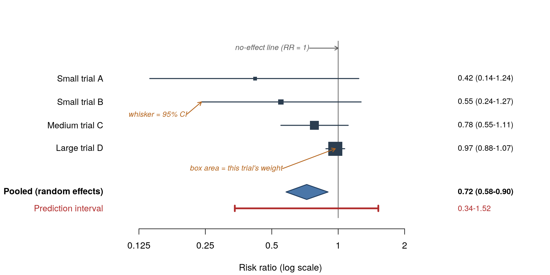
Six things to check, in this order:
- Where is the diamond, and does it cross the null line? That is the headline.
- Where is the prediction interval? If it crosses the null while the diamond does not, the average effect is positive but a new setting could easily see nothing.
- Are the big boxes and the small boxes on the same side? If the large trials sit near the null and the small ones sit far from it, stop and read Section 24.10 before believing the diamond.
- Do the whiskers overlap? Non-overlapping intervals mean the studies genuinely disagree.
- Is one box doing all the work? A single dominant trial means you have one trial with decoration, not a meta-analysis.
- Heterogeneity statistics, which the plot usually prints along the bottom.
Now the real thing:
Code
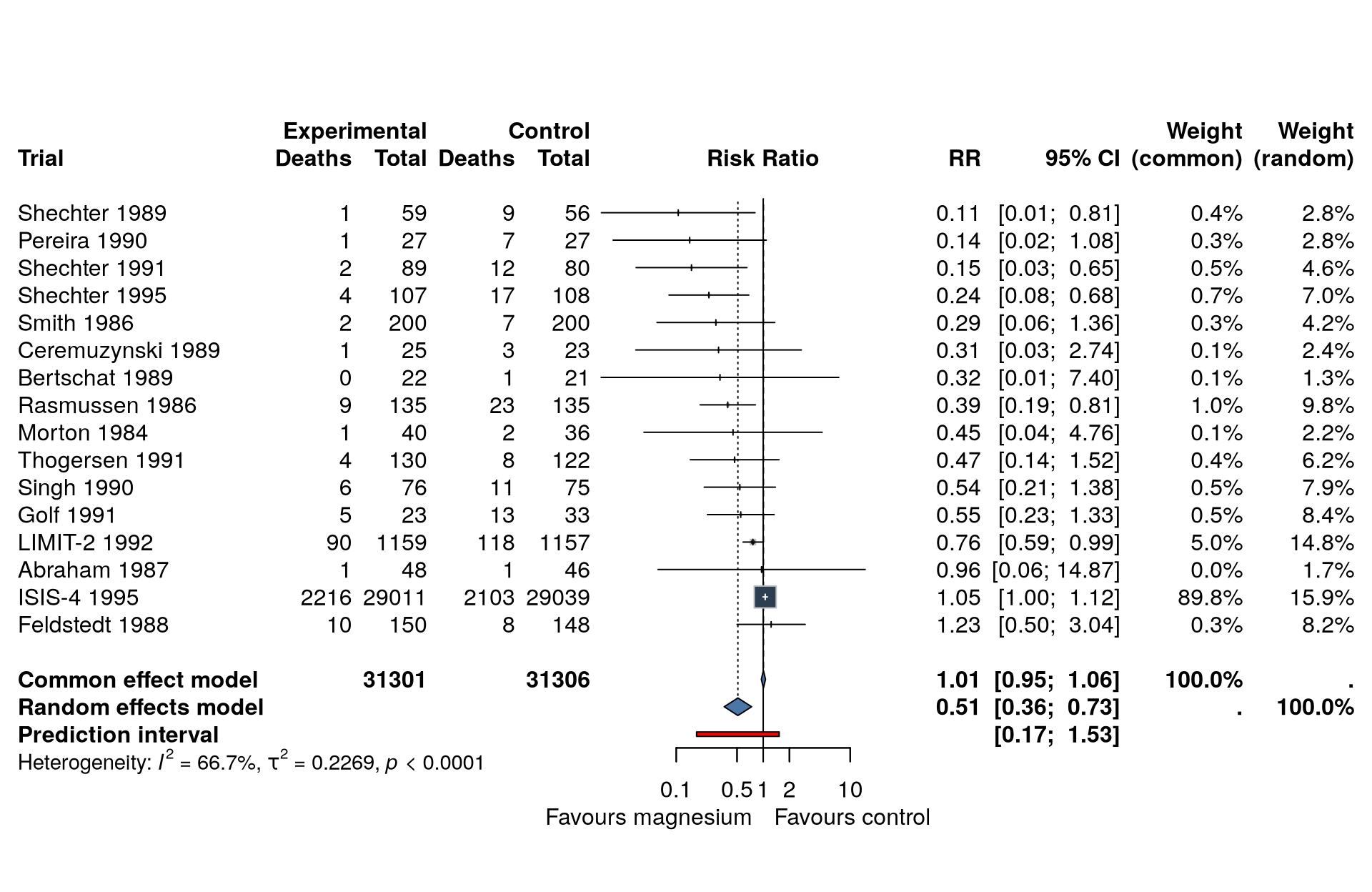
What to notice. Apply check 3 from the list. Fourteen of the fifteen smaller trials sit left of the null line — several of them far left, with risk ratios of 0.11 to 0.24 — while the one very large trial sits astride it at 1.05. That pattern, effect size shrinking as trials get bigger, has a name: small-study effects. It is the single most useful thing a forest plot can show you.
meta also prints two weight columns, and they are worth a moment. ISIS-4 carries 89.8% of the weight under the common-effect model and 15.9% under random effects. The mechanism from the callout above is right there in the output: the same trial, the same data, an 80-percentage-point swing in influence purely from adding \(\hat{\tau}^2\) to the denominator.
24.7 Heterogeneity: What Actually Varies
Heterogeneity means the studies disagree more than chance alone would explain. A tidy pooled estimate can hide wide disagreement underneath, so quantifying it tells you how much to trust the average.
Three statistics get reported, and they answer three genuinely different questions. Confusing them is the most common error in the meta-analysis literature (Borenstein 2024).
| Statistic | The question it answers | What it is not |
|---|---|---|
| Cochran’s \(Q\) (and its p-value) | Is there any real variation at all? A hypothesis test. | Not a measure of how much variation there is. Underpowered with few studies; over-powered with many. |
| \(I^2\) | What proportion of the observed scatter is real rather than sampling noise? | Not how much the effect varies. A relative quantity: it can be 90% with trivial variation, or 0% with large variation, depending on how precise the studies are. |
| \(\tau^2\) / \(\tau\) | How much do the true effects vary? An absolute measure, on the effect scale. | Hard to interpret directly on a log scale. |
All three are built from one quantity, \(Q\), so it is worth taking that apart slowly.
\[ \underbrace{Q}_{\substack{\text{total observed} \\ \text{disagreement}}} \;=\; \sum_{i=1}^{k} \underbrace{w_i^{\text{FE}}}_{\substack{\text{precise studies} \\ \text{count for more}}} \times \underbrace{\left(\hat{\theta}_i - \hat{\theta}_{\text{FE}}\right)^2}_{\substack{\text{squared distance from} \\ \text{the pooled estimate}}} \]
Term by term:
- \((\hat{\theta}_i - \hat{\theta}_{\text{FE}})^2\) is how far study \(i\) landed from the pooled result, squared — so that falling short and overshooting both count as disagreement.
- Multiplying by \(w_i^{\text{FE}} = 1/\hat{\sigma}_i^2\) says that a precise study sitting far from the pooled estimate is more surprising than an imprecise one doing the same. Each term is therefore a distance measured in units of that study’s own noise.
- That scaling is what makes \(Q\) interpretable. If every study really were estimating the same effect, each term would average about 1, so the whole sum would average about \(k - 1\) (one degree of freedom goes on estimating the pooled effect itself). So compare \(Q\) with \(k-1\): the excess is disagreement that sampling noise cannot account for. On the magnesium data \(Q = 45.1\) against \(k - 1 = 15\) — three times what noise alone would produce, hence \(p = 0.0001\).
Both summary statistics are then built from that same excess, \(Q - (k-1)\):
\[ I^2 = \frac{\overbrace{Q - (k-1)}^{\text{excess over noise}}}{\underbrace{Q}_{\text{total disagreement}}} \times 100\% \qquad\qquad \hat{\tau}^2 = \frac{\overbrace{Q - (k-1)}^{\text{excess over noise}}}{\underbrace{C}_{\substack{\text{scaling constant} \\ \text{(see below)}}}} \]
where \(C = \sum_i w_i - \left(\sum_i w_i^2 \big/ \sum_i w_i\right)\), and both quantities are set to zero if the excess comes out negative, which sampling noise alone can produce. (This is the DerSimonian-Laird version of \(\hat{\tau}^2\), the one you can compute by hand; REML, which is preferred, solves for it iteratively instead.)
Same numerator, different denominators — and that is the entire distinction between the two. Dividing the excess by \(Q\) gives a proportion: what share of the disagreement we can see is real rather than noise (66.7% here). Dividing it instead by \(C\) rescales the excess into a variance on the effect scale (0.174 by this formula, 0.227 by REML), which is an amount rather than a share. This is why \(I^2\) can be large when the true effects barely differ and small when they differ a lot: recruit ten times as many patients per trial and \(Q\) — the denominator — grows, so \(I^2\) rises, without the true effects having moved at all.
Important\(I^2\) does not tell you how much the effect varies
You will see the 25% / 50% / 75% “low / moderate / high” thresholds everywhere, including in Higgins et al. (2003) where they were offered as tentative rules of thumb. Current methodological guidance is blunt about them: classifications of heterogeneity based on \(Q\), its p-value, or \(I^2\) are “uninformative at best, and often misleading” (Borenstein 2024, 2023).
The reason is that \(I^2\) is a ratio, not an amount. It is the share of observed scatter that is real rather than noise. Run the same trials with ten times as many patients each and the sampling noise shrinks, so \(I^2\) rises — without the true effects having moved at all.
The statistic that answers “how much does the effect vary?” is the prediction interval. Report it. Use \(I^2\), if at all, only to say what fraction of the scatter is signal.
24.7.1 The prediction interval
The confidence interval describes the average true effect. The prediction interval answers the question a clinician actually has: if this treatment were used in a new setting tomorrow, what range of true effects might we see?
\[ \underbrace{\hat{\mu}}_{\substack{\text{estimated average} \\ \text{true effect}}} \;\pm\; \underbrace{t_{k-2,\,0.975}}_{\substack{\text{multiplier, } k-2 \text{ degrees}\\ \text{of freedom (we estimated}\\ \text{both } \mu \text{ and } \tau^2)}} \times \underbrace{\sqrt{\underbrace{\text{SE}(\hat{\mu})^2}_{\substack{\text{we are unsure} \\ \text{of the average}}} + \underbrace{\hat{\tau}^2}_{\substack{\text{settings genuinely} \\ \text{differ}}}}}_{\substack{\text{total spread of a new} \\ \text{setting's true effect}}} \]
Read it as three pieces.
\(\hat{\mu}\), the centre, is just the random-effects pooled estimate — the same number the confidence interval is built around. A prediction interval is not a different estimate; it is the same estimate with a wider ruler.
The square-root term is where the intuition lives. There are two independent reasons a new setting’s true effect might not equal \(\hat{\mu}\): we do not know \(\mu\) exactly (that is \(\text{SE}(\hat{\mu})^2\)), and the truth genuinely differs from place to place even if we did know \(\mu\) (that is \(\hat{\tau}^2\)). Independent uncertainties add as variances, not as widths — the same reason a journey made of two uncertain legs is less uncertain than the sum of its two worst cases — so the two terms are added under the square root rather than added directly. A useful consequence: whichever term is much the larger dominates. Here \(\text{SE}(\hat{\mu})^2 = 0.036\) against \(\hat{\tau}^2 = 0.227\), so roughly six-sevenths of the width comes from genuine between-setting variation, not from our ignorance about the average.
The \(t\) multiplier plays the role that 1.96 plays in an ordinary confidence interval, but it is larger, because \(\hat{\tau}^2\) is itself an estimate from only \(k\) studies. With 16 trials it is 2.15 rather than 1.96; with 5 trials it would be 3.18. Few studies means an untrustworthy estimate of how much settings differ, and the multiplier says so.
The extra \(\hat{\tau}^2\) under the square root is the whole point, and it is why the prediction interval in Figure 24.2 is drawn wider than the diamond: the confidence interval shrinks towards zero width as you add studies, because \(\text{SE}(\hat{\mu})\) does, but the prediction interval does not, because real between-setting variation does not go away no matter how precisely you measure it (Riley et al. 2011; IntHout et al. 2016). An infinite number of studies would tell you the average effect exactly and still leave you unsure what the next hospital will see.
NoteWhich prediction-interval formula your software uses
The form above is the original one (Riley et al. 2011), and it is what the Python tab computes by hand. meta 8.x defaults to a refinement (method.predict = "V") that uses \(k-1\) degrees of freedom and a slightly different variance for \(\hat{\mu}\), on the grounds of better coverage (Partlett and Riley 2017). On these data the two agree closely — 0.170 to 1.536 versus 0.171 to 1.526 — and the choice between them matters far less than reporting an interval at all. Say which you used.
For the magnesium data:
| \(\tau^2\) | 0.227 (so \(\tau = 0.48\) on the log-RR scale — substantial) |
| \(I^2\) | 66.7% |
| \(Q\) test | p = 0.0001 |
| Pooled RR (random effects) | 0.511 (95% CI 0.356 to 0.735) |
| Prediction interval | 0.171 to 1.526 |
Read the last two rows together. The confidence interval says the average effect is a clear benefit. The prediction interval includes 1 — so on this evidence, a new trial could plausibly find magnesium halves mortality, or that it does nothing, or that it causes modest harm. A guideline committee shown only the confidence interval would draw a very different conclusion from one shown both.
24.8 Investigating Heterogeneity
When heterogeneity is substantial, the useful question is not “how big is \(I^2\)” but “what differs between these studies?” A characteristic that might explain the differences is called a moderator. It is a property of the study, not of an individual patient: the year the trial ran, the dose used, the average age of the population it recruited, its risk-of-bias rating.
There are two ways to test a moderator, and they are one idea applied to two kinds of variable.
Subgroup analysis is for a categorical moderator. Split the studies into groups — trials in hospital settings versus trials in primary care, high dose versus low dose — pool each group separately, then test whether the group estimates differ by more than chance. It answers: does the effect differ between these kinds of study?
Meta-regression is for a continuous moderator. Rather than splitting, it fits a weighted straight line across the studies, with the moderator on the horizontal axis and each study’s effect estimate on the vertical, again giving precise studies more say. The slope says how much the effect changes per unit of the moderator — “the log risk ratio rose by 0.05 for each later calendar year”. It answers: does the effect trend with this quantity?
The two are faces of the same model: a subgroup analysis with two groups is a meta-regression on a 0/1 indicator, and the test for a subgroup difference is the test of that indicator’s slope. Choose subgroups when the moderator really is categorical, and meta-regression when chopping a continuous variable at an arbitrary cut-point would throw information away — the same argument Chapter 5 makes for patient-level data.
Two constraints on both. They should be pre-specified: with a handful of studies and a free choice of moderator, you will always find something. And you have far less power than the patient counts suggest, because the unit of analysis is the study, not the patient — 16 trials give you 16 data points for the line. A common rule of thumb is at least ten studies per moderator examined (Higgins et al. 2024).
Code
library(meta)
library(metafor)

# --- meta-regression on calendar year -------------------------------------
es <- escalc(measure = "RR", ai = ai, n1i = n1i, ci = ci, n2i = n2i,
             data = dat.egger2001)
mr <- rma(yi, vi, mods = ~ I(year - 1984), data = es, method = "REML")
cat(sprintf("year slope: %+.4f log RR per year, p = %.3f, R^2 = %.0f%%\n",
            mr$beta[2], mr$pval[2], mr$R2))

# --- subgroup analysis by trial size --------------------------------------
es$size <- ifelse(es$n1i + es$n2i < 400, "small (<400)", "large (>=400)")
m_sub <- update(m, subgroup = es$size)
m_sub
What the code shows and what it finds. The meta-regression asks whether the effect drifted over calendar time: the slope is \(+0.052\) log-RR per year with p = 0.37, explaining only 13% of the heterogeneity. On its own that is a null result, and it would be easy to report it as “no evidence of a time trend” and move on.
Splitting by trial size instead tells a different story:
| Subgroup | Trials | Pooled RR (random effects) |
|---|---|---|
| Small (<400 patients) | 13 | 0.423 (0.284 to 0.630) |
| Large ($$400 patients) | 3 | 0.869 (0.362 to 2.085) |
| Test for subgroup difference | p = 0.0085 |
The small trials say magnesium more than halves mortality. The large trials say it probably does nothing. And these two moderators are entangled — the large trials are also the later ones — which is why the year analysis picked up a weak, non-significant signal for what is really a size effect. A non-significant moderator does not mean there is no explanation for the heterogeneity; it can mean you chose the wrong moderator.
WarningTwo cautions on this subgroup analysis
First, the honest one: splitting by trial size is a diagnostic, not a pre-specified subgroup analysis. Size is not a patient characteristic and there is no clinical hypothesis attached to it. It belongs in the small-study-effects investigation below, not in the results table as a subgroup finding.
Second, the ecological fallacy. Study-level associations do not imply individual-level ones. If trials with older populations show larger effects, that does not establish that older individuals benefit more — the trials may differ in a dozen other ways. This is a fundamental limitation of aggregate-data meta-analysis, and the reason individual participant data (Section 24.12) is worth the effort when the question is about who benefits.
24.9 Bayesian Meta-Analysis
You have already met everything needed for this. A random-effects meta-analysis is a hierarchical model — statisticians call this particular one the normal-normal hierarchical model — which is exactly the object Chapter 10 introduced, so the Bayesian version is not a new method. It is the same two lines of model, fitted the way that chapter fitted things (Sutton and Abrams 2001).
Written out, the model is:
\[ \underbrace{\hat{\theta}_i \sim N(\theta_i,\; \hat{\sigma}_i^2)}_{\substack{\text{what we observe: each study's estimate} \\ \text{scatters around its own true effect}}} \qquad\qquad \underbrace{\theta_i \sim N(\mu,\; \tau^2)}_{\substack{\text{what we assume: the true effects} \\ \text{scatter around an average}}} \]
The second line is the random-effects assumption from earlier in this chapter, unchanged. The difference is what happens to \(\mu\) and \(\tau\). The frequentist route estimates \(\tau^2\) once, by REML, and then treats that single number as though it were known when computing everything downstream — the Hartung-Knapp adjustment is a partial patch for exactly this (IntHout et al. 2014). The Bayesian route puts a prior on \(\mu\) and on \(\tau\) and returns a joint posterior, so uncertainty about how much studies differ is carried through to every number you report. This is the main argument Higgins et al. (2009) make for the approach, and the reason it is standard practice when studies are few (Röver et al. 2021).
Three things you get for the trouble:
- Honest uncertainty about \(\tau\). With few studies, \(\tau^2\) is the weakest quantity in a meta-analysis, and the frequentist interval’s coverage suffers for it. A posterior gives you an interval for \(\tau\) instead of a point.
- Direct probability statements. “There is a 99% probability the risk ratio is below 1” is a sentence a frequentist analysis cannot produce, and a clinician immediately understands.
- The prediction interval for free. Draw \(\mu\) and \(\tau\) from the posterior, then draw a new \(\theta_{\text{new}} \sim N(\mu, \tau^2)\) for each — and you have the distribution of the true effect in a new setting (Section 24.7.1), with no \(t\) approximation needed. Higgins et al. (2009) argue this predictive distribution, not the confidence interval for \(\mu\), is the result a random-effects meta-analysis should lead with.
Code
library(brms)      # installed by scripts/post_install.sh, not from conda;
library(metafor)   # needs a working C++ toolchain (see the setup chapter)

# escalc() turns the 2x2 counts into log risk ratios (yi) and their variances
# (vi); it adds 0.5 to the trial with a zero cell, as metabin() did.
es <- escalc(measure = "RR", ai = ai, n1i = n1i, ci = ci, n2i = n2i,
             data = dat.egger2001)
es$sei   <- sqrt(es$vi)
es$trial <- paste(es$study, es$year)

# yi | se(sei)  -- the outcome is an estimate whose standard error we already
#                  know, so brms should not try to estimate residual noise
# (1 | trial)   -- each trial gets its own true effect; the SD of these IS tau
fit <- brm(
  yi | se(sei) ~ 1 + (1 | trial),
  data  = es,
  prior = c(prior(normal(0, 1),   class = Intercept),  # prior on mu
            prior(normal(0, 0.5), class = sd)),        # prior on tau (half-normal)
  chains = 4, iter = 4000, warmup = 1000, seed = 24,
  control = list(adapt_delta = 0.95)
)

draws <- as_draws_df(fit)
mu  <- draws$b_Intercept            # average log risk ratio
tau <- draws$sd_trial__Intercept    # between-study SD

cat(sprintf("Pooled RR %.3f (95%% CrI %.3f to %.3f)\n",
            exp(median(mu)), exp(quantile(mu, .025)), exp(quantile(mu, .975))))
cat(sprintf("tau       %.3f (95%% CrI %.3f to %.3f)\n",
            median(tau), quantile(tau, .025), quantile(tau, .975)))
cat(sprintf("P(RR < 1) = %.3f   P(RR < 0.9) = %.3f\n",
            mean(mu < 0), mean(mu < log(0.9))))

# Posterior predictive effect in a NEW setting = the prediction interval.
# One draw of theta_new per posterior draw of (mu, tau), so the interval carries
# uncertainty about tau rather than fixing it at a point estimate.
set.seed(24)
theta_new <- rnorm(length(mu), mu, tau)
cat(sprintf("New-setting interval: %.3f to %.3f\n",
            exp(quantile(theta_new, .025)), exp(quantile(theta_new, .975))))
Two notes on the priors, since they are the only genuinely new decision here.
normal(0, 1) on \(\mu\) is on the log scale, so it says the risk ratio is probably somewhere between about 0.14 and 7 — wide enough to be uninformative about any plausible clinical effect.
normal(0, 0.5) on class = sd is automatically truncated at zero by brms, making it a half-normal prior on \(\tau\) with scale 0.5. That is not an arbitrary choice: the half-normal family is the one generally recommended for \(\tau\) in this model, and for effect measures on a log scale a scale of 0.5 is the specific weakly informative default that Röver et al. (2021) arrive at — it puts most of its mass on heterogeneity in the “reasonable to fairly high” range and only 4.6% above \(\tau = 1\). It expects some heterogeneity while treating a great deal of it as unlikely. With few studies this prior does real work, and the better move is then an informative one drawn from the empirical distribution of \(\tau\) across comparable meta-analyses (Turner et al. 2012) rather than any generic default.
What the code shows. The Bayesian and frequentist answers land in nearly the same place:
| Bayesian (brms) | Frequentist (REML + Hartung-Knapp) | |
|---|---|---|
| Pooled RR | 0.541 (95% CrI 0.347 to 0.781) | 0.511 (95% CI 0.356 to 0.735) |
| \(\tau\) | 0.459 (95% CrI 0.217 to 0.837) | 0.476 (point estimate) |
| Effect in a new setting | 0.168 to 1.537 | 0.171 to 1.526 |
| \(P(\text{RR} < 1)\) | \(> 0.999\) | not available |
Look at the \(\tau\) row: the frequentist analysis reports one number, the Bayesian one reports 0.22 to 0.84. Between-study variation could be half what REML estimated or nearly double it, and that is the uncertainty the prediction interval depends on. With sixteen studies the two approaches agree closely, which is the expected result and a good sanity check. With five studies they would not, and the Bayesian version would be the more honest of the two.
Because the prior on \(\tau\) matters most when it matters at all, refit with a different one and report both:
Barely moves — with sixteen studies the data, not the prior, is deciding. That sentence is only worth writing because you checked.
WarningWhat the Bayesian version does not fix
Read that \(P(\text{RR} < 1) > 0.999\) again. The model is more than 99.9% certain that magnesium reduces mortality after a heart attack.
It is wrong, and the next section explains why. Priors express uncertainty about parameters; they say nothing about studies that were run and never published. Any model — REML, Hartung-Knapp, Bayesian, whatever comes next — fitted to a biased set of studies returns a confident, well-calibrated-looking answer about the wrong quantity. A more careful model is not a substitute for a more complete set of studies.
24.10 Small-Study Effects and Non-Reporting Bias
NoteA note on terminology
This used to be called “publication bias”. Current Cochrane guidance prefers non-reporting bias, because studies go missing for several reasons besides never being published — selective reporting of outcomes, language restrictions, delayed publication — and because the funnel plot detects the symptom (small-study effects) rather than the cause (Higgins et al. 2024).
Studies with positive, statistically significant results are more likely to be published, published sooner, and published in English. If the unremarkable trials are sitting in a drawer, the evidence you can see is skewed towards good news.
24.10.1 Funnel plots
A funnel plot puts each study’s effect estimate on the horizontal axis and its standard error on the vertical axis, upside down, so the most precise studies sit at the top.
That vertical axis is study size in disguise. A standard error shrinks roughly in proportion to \(1/\sqrt{n}\), so a trial with four times as many patients has half the standard error. Big trials therefore have small standard errors and sit near the top of the plot; small trials have large ones and sit near the bottom.
Why the boundary lines are diagonal. Suppose every study really is estimating the same effect. A study with standard error SE would then land within roughly \(\pm 1.96 \times \text{SE}\) of that common effect 95% of the time. Now read that as you move down the plot: at the very top SE is nearly zero, so the scatter a study is allowed is nearly zero; halfway down, SE is half its largest value, so the allowed scatter is half as wide as at the bottom. The permitted spread grows in direct proportion to SE — and a quantity growing in direct proportion draws a straight line. Two of them, one per side, meeting at the apex: a triangle, or an inverted funnel.
With no small-study effects, the studies should fill that triangle symmetrically — a tight cluster at the top, fanning out evenly to left and right further down. It is the asymmetry, not the funnel shape itself, that you are looking for.
Code
# The three reference lines are deliberately styled to be told apart: the funnel
# edges and the fixed-effect line share a grey dashed look (the funnel is drawn
# around the fixed-effect estimate), while the random-effects estimate is solid
# red. ref = NA suppresses meta's no-effect line, which here would sit almost
# exactly on top of the fixed-effect line (1.006 versus 1.000) and add nothing
# but confusion.
funnel(m,
  xlab = "Risk ratio (log scale)",
  ylab = "Standard error (larger trials sit higher up)",
  level = 0.95,        # draw the pseudo-95% confidence funnel
  studlab = FALSE,
  bg = "#2c3e50", col = "black",
  col.common = "grey50", lty.common = 2, lwd.common = 1.6,
  col.random = "#b02a2a", lty.random = 1, lwd.random = 1.8,
  ref = NA
)
legend("topleft", bty = "n", cex = 0.8, inset = c(0, 0.03),
       legend = c("Fixed effect (1.01) + 95% funnel", "Random effects (0.51)"),
       col = c("grey50", "#b02a2a"), lty = c(2, 1), lwd = c(1.6, 1.8))
# Note: funnel() plots on the risk-ratio scale with a log axis, so annotation
# coordinates are risk ratios, not log risk ratios.
text(3.5, 1.30, "the small trials that\nfound nothing are\nnot here",
     col = "grey35", cex = 0.8, font = 3)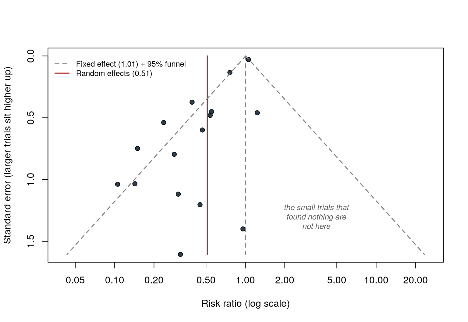
Code
import numpy as np
import matplotlib.pyplot as plt

se = np.sqrt(var)
fig, ax = plt.subplots(figsize=(7.5, 5.5))

# The pseudo-95% funnel: +-1.96 SE either side of the fixed-effect estimate,
# traced down the range of standard errors. This is the line that makes the
# triangle -- the wider a study's SE, the further it is allowed to scatter.
se_grid = np.linspace(0.001, se.max() * 1.05, 100)
ax.fill_betweenx(se_grid, te_fe - 1.96 * se_grid, te_fe + 1.96 * se_grid,
                 color="#eff2f5", zorder=0)
ax.plot(te_fe - 1.96 * se_grid, se_grid, color="grey", lw=1.3, ls="--", zorder=1)
ax.plot(te_fe + 1.96 * se_grid, se_grid, color="grey", lw=1.3, ls="--", zorder=1,
        label="95% funnel around the fixed-effect estimate")

# Two estimates, styled so they cannot be mistaken for each other or the funnel
ax.axvline(te_fe, color="grey", lw=1.4, ls="--", zorder=2,
           label=f"Fixed effect ({np.exp(te_fe):.2f})")
ax.axvline(te_re, color="#b02a2a", lw=1.8, ls="-", zorder=2,
           label=f"Random effects ({np.exp(te_re):.2f})")

ax.scatter(log_rr, se, s=30, color="#2c3e50", zorder=3, label="Trials")
ax.invert_yaxis()                     # most precise (largest) studies at the top
ax.set_xlabel("log risk ratio")
ax.set_ylabel("Standard error (larger trials sit higher up)")
ax.set_title("Funnel plot: magnesium trials")
ax.legend(loc="upper left", frameon=False, fontsize=8)
plt.tight_layout()
plt.show()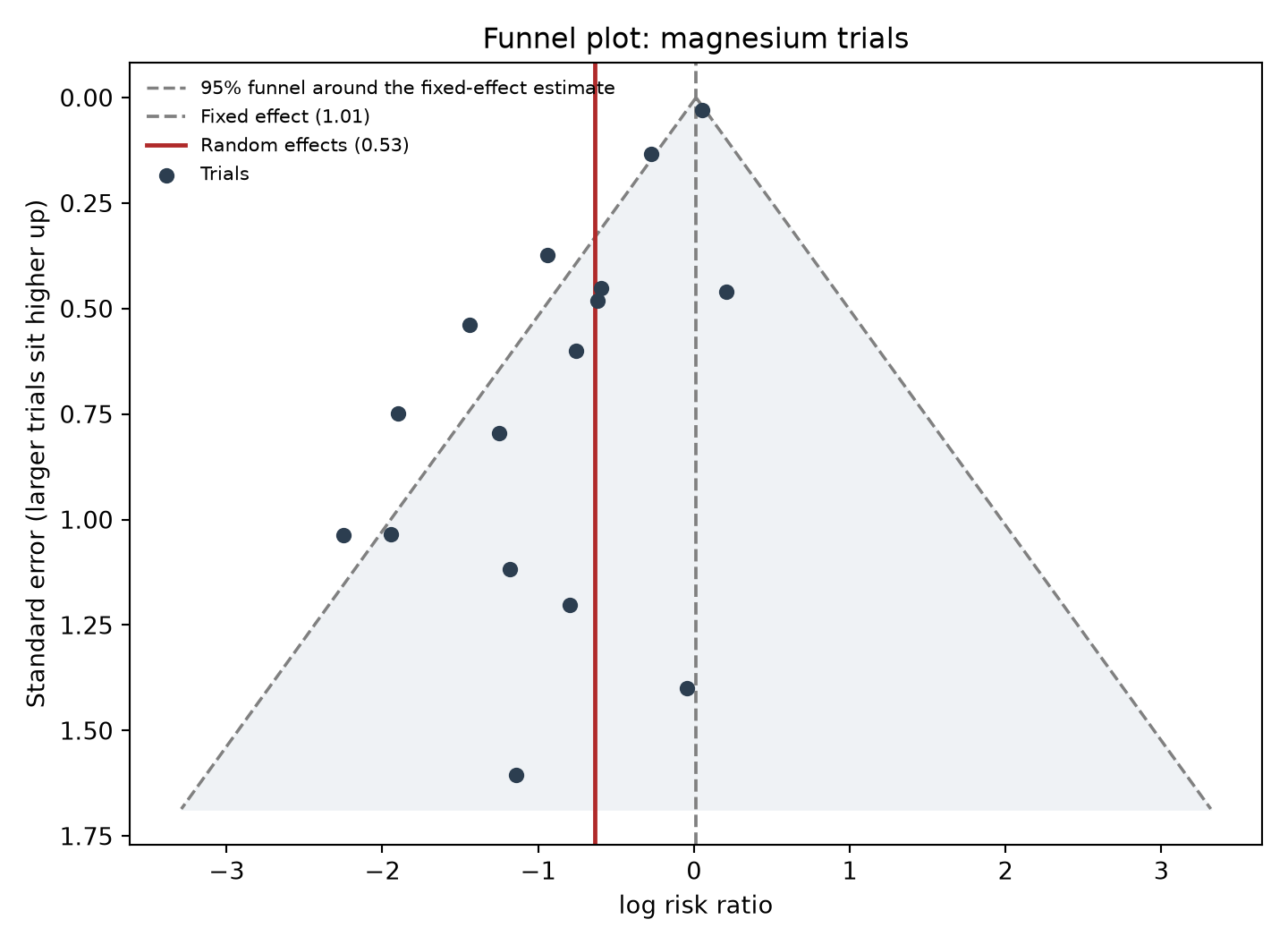
The asymmetry is stark. Look at the bottom of the plot, where the imprecise little trials live: the left side (benefit) is populated and the right side (no benefit or harm) is nearly empty. Either small trials of magnesium happened to work much better than large ones, or the small trials that found nothing were never published.
24.10.2 Testing for asymmetry — and choosing the right test
You can turn the eyeball judgement into a number, with two important constraints.
Constraint one: you need at least 10 studies. Below that, the tests have too little power to distinguish chance from real asymmetry, and Cochrane advises against using them at all (Higgins et al. 2024). This threshold is rarely met in practice, so most published meta-analyses cannot legitimately test for asymmetry. Saying “we could not assess it” is the correct report, not “the test was non-significant”.
Constraint two: the standard test is wrong for some effect measures. Egger’s test regresses the effect estimate on its standard error (Egger et al. 1997). For odds ratios and standardised mean differences, the standard error is mathematically linked to the size of the effect, which produces funnel-plot asymmetry and small p-values even when nothing is missing. Cochrane therefore recommends the Harbord (Harbord et al. 2006) or Peters (Peters et al. 2006) tests for binary outcomes instead.
What the code shows. All three agree emphatically — Egger p < 0.0001, Harbord p = 0.0001, Peters p = 0.0023. The Peters test is the most conservative of the three, which is the usual pattern and a reason to prefer it when the outcome is binary. When the tests disagree, believe the one appropriate to your effect measure, not the one with the smallest p-value.
WarningTrim-and-fill: know it, do not lean on it
You will meet trim-and-fill, which imputes the “missing” studies needed to make the funnel symmetric and then re-pools. On these data it adds 8 imputed trials and moves the estimate from RR 0.51 to 0.90 (95% CI 0.52 to 1.54) — in this case, closer to the truth.
Do not take that as an endorsement. Trim-and-fill assumes one specific mechanism for why studies are missing, it does not estimate what the absent studies actually found, and it is not among the methods in current Cochrane guidance (Higgins et al. 2024). Treat it as a sensitivity analysis that shows how fragile the pooled estimate is, never as a bias-corrected result.
24.10.3 What actually happened
The historical answer is known, and it is why this dataset is worth your time.
The first seven trials were pooled in the early 1990s, then combined with LIMIT-2 (1,159 patients) in a 1993 meta-analysis that concluded magnesium was an effective, cheap treatment for acute myocardial infarction. Some clinicians adopted it.
Then ISIS-4 reported: 58,050 randomised patients, the largest trial in the set, and a mortality risk ratio of 1.055 — no benefit, if anything slight harm (ISIS-4 Collaborative Group 1995).
The small trials were wrong. A meta-analysis of them was confidently, publishably wrong, and the funnel plot in Figure 24.4 was visible years before ISIS-4 reported. The lesson is not that meta-analysis is untrustworthy; it is that a pooled estimate is only as good as the set of studies you can see, and that the diagnostics in this chapter exist because that set is often incomplete.
Everything in the standard analysis pointed at this, if you read it properly: a fixed-versus-random gap of 1.006 versus 0.511, a prediction interval crossing 1, and three asymmetry tests with p < 0.01.
24.11 Reporting a Meta-Analysis
Follow PRISMA 2020 (Page et al. 2021) for the review: the 27-item checklist, the flow diagram of records screened and excluded, and a pre-registered protocol (PROSPERO).
For the analysis itself, report these four things together. A pooled estimate on its own is not interpretable:
- The pooled effect with its confidence interval, and which model produced it.
- \(\tau^2\) (or \(\tau\)) and the prediction interval. Not just \(I^2\) — see Section 24.7.
- The methods you chose and why: the \(\tau^2\) estimator, the confidence-interval method, and how you handled zero cells.
- What you could and could not assess. If you had fewer than 10 studies, say that you could not evaluate small-study effects, rather than reporting a non-significant test.
Certainty of evidence is usually summarised with GRADE, which downgrades for risk of bias, inconsistency (heterogeneity), indirectness, imprecision, and publication bias. Most clinical journals now expect a GRADE summary-of-findings table alongside the meta-analysis; it is a separate skill from the statistics and worth learning from the GRADE handbook directly.
24.12 Where to Go Next
This chapter deliberately stops at aggregate-data meta-analysis of one comparison. The methods below are each a chapter in their own right; here is what they are for and where to start.
| Method | The question it answers | Where to start |
|---|---|---|
| Network meta-analysis | Which of several treatments is best, when few have been compared head to head? Combines direct and indirect evidence. | netmeta in R; Salanti (2012). Check the network is connected and that transitivity is plausible before believing any ranking. |
| Individual participant data (IPD) meta-analysis | Who benefits? Needs raw patient-level data from each study, which avoids the ecological fallacy. | Riley et al. (2019), Riley et al. (2020); one-stage mixed models or two-stage pooling. |
| Bayesian meta-analysis (covered in Section 24.9) | The same random-effects model, but with a prior on \(\tau\) — which is what you want when there are too few studies to estimate heterogeneity well. | bayesmeta in R is a lighter alternative to the brms fit shown above; for informative priors on \(\tau\), see Turner et al. (2012). |
| Dose-response meta-analysis | Is there a gradient rather than a yes/no effect? | dosresmeta in R. |
| Prognostic and prediction-model reviews | Does a published model work elsewhere? | Riley et al. (2019); connects directly to Chapter 18. |
For everything in this chapter, Harrer et al. (2021) is the best free code-first companion and goes considerably deeper than we do here.
24.13 Exercises
TipExercise 1: Fixed versus random effects, and why it mattered
Load dat.egger2001 from metafor and reproduce the core analysis.
- Pool the sixteen trials with a fixed-effect and then a random-effects model (REML, Hartung-Knapp interval). Report both risk ratios.
- Compute each trial’s percentage weight under each model. How much weight does ISIS-4 carry under each, and why does it change so much?
- Report \(\tau^2\), \(I^2\), and the prediction interval. Which of the three tells a clinician how much the effect varies between settings?
- In one sentence each, write what you would tell a guideline committee based on (i) the fixed-effect result alone and (ii) the random-effects result alone.
NoteSolution
Code
# =============================================================================
# Chapter 18 - Exercise 1: Fixed versus random effects, and why it mattered
# Intravenous magnesium after acute myocardial infarction (16 trials)
# =============================================================================
#
# Libraries -------------------------------------------------------------------
library(meta)     # metabin()
library(metafor)  # the dat.egger2001 dataset
library(tidyverse)

d <- dat.egger2001

# Note: in this dataset the control-arm event count is called `ci`, which reads
# confusingly next to "confidence interval". It is deaths in the control arm.
m <- metabin(
  event.e = ai, n.e = n1i,     # deaths / patients on magnesium
  event.c = ci, n.c = n2i,     # deaths / patients on control
  studlab = paste(study, year),
  data = d,
  sm = "RR",
  method.tau = "REML",         # REML rather than DerSimonian-Laird
  method.random.ci = "HK",     # Hartung-Knapp-Sidik-Jonkman interval
  prediction = TRUE
)

rr <- function(x) exp(x)

# -----------------------------------------------------------------------------
# (a) Both models
# -----------------------------------------------------------------------------
cat("=== (a) Fixed-effect vs random-effects ===\n")
cat(sprintf("Fixed effect   RR = %.3f (95%% CI %.3f to %.3f)\n",
            rr(m$TE.common), rr(m$lower.common), rr(m$upper.common)))
cat(sprintf("Random effects RR = %.3f (95%% CI %.3f to %.3f)\n",
            rr(m$TE.random), rr(m$lower.random), rr(m$upper.random)))
cat("\nSame 16 trials, same outcome. One model says magnesium does nothing;\n")
cat("the other says it roughly halves mortality.\n")

# -----------------------------------------------------------------------------
# (b) Where did the weight go?
# -----------------------------------------------------------------------------
w <- tibble(
  trial = m$studlab,
  n = d$n1i + d$n2i,
  fixed_pct = 100 * m$w.common / sum(m$w.common),
  random_pct = 100 * m$w.random / sum(m$w.random)
) |>
  arrange(desc(n))

cat("\n=== (b) Percentage weight under each model ===\n")
print(as.data.frame(w |> mutate(across(ends_with("pct"), \(x) round(x, 1)))),
      row.names = FALSE)

isis <- w |> filter(str_detect(trial, "ISIS"))
cat(sprintf(
  "\nISIS-4 has %.0f%% of all the patients but carries %.1f%% of the weight under\n",
  100 * isis$n / sum(w$n), isis$fixed_pct
))
cat(sprintf("the fixed-effect model and only %.1f%% under random effects.\n",
            isis$random_pct))
cat("\nWhy: random-effects weights are 1 / (within-study variance + tau^2).\n")
cat("ISIS-4's within-study variance is tiny, so adding tau^2 = ", round(m$tau2, 3),
    "\nswamps it and its weight collapses. A small trial's variance is already\n")
cat("large, so the same addition barely changes it. The effect is to level the\n")
cat("weights -- which hands the analysis to the 13 small trials.\n")

# -----------------------------------------------------------------------------
# (c) Heterogeneity: three statistics, three different questions
# -----------------------------------------------------------------------------
cat("\n=== (c) Heterogeneity ===\n")
cat(sprintf("tau^2 = %.3f  (tau = %.3f on the log-RR scale)\n", m$tau2, sqrt(m$tau2)))
cat(sprintf("I^2   = %.1f%%   Q test p = %.4f\n", 100 * m$I2, m$pval.Q))
cat(sprintf("Prediction interval: %.3f to %.3f\n",
            rr(m$lower.predict), rr(m$upper.predict)))
cat("\nThe PREDICTION INTERVAL is the one that answers 'how much does the effect\n")
cat("vary between settings'. I^2 is a ratio -- the share of the observed scatter\n")
cat("that is real rather than sampling noise -- and would rise if you simply ran\n")
cat("the same trials with more patients each. Note that the prediction interval\n")
cat("INCLUDES 1, while the confidence interval does not.\n")

# -----------------------------------------------------------------------------
# (d) What you would tell a guideline committee
# -----------------------------------------------------------------------------
cat("\n=== (d) Two one-sentence summaries ===\n")
cat("(i)  Fixed effect only: \"Pooling 62,607 patients across 16 randomised\n")
cat("     trials, intravenous magnesium had no effect on mortality after\n")
cat("     myocardial infarction (RR 1.01, 95% CI 0.95 to 1.06).\"\n\n")
cat("(ii) Random effects only: \"Pooling 16 randomised trials, intravenous\n")
cat("     magnesium reduced mortality after myocardial infarction by almost\n")
cat("     half (RR 0.51, 95% CI 0.36 to 0.74).\"\n\n")
cat("Both sentences are defensible from the same data, which is exactly why you\n")
cat("must report both models when they disagree, and why the prediction interval\n")
cat("and the funnel plot are not optional extras.\n")
Code
# =============================================================================
# Chapter 18 - Exercise 1: Fixed versus random effects, and why it mattered
# Intravenous magnesium after acute myocardial infarction (16 trials)
# =============================================================================

# Libraries -------------------------------------------------------------------
# pip install numpy pandas scipy
import numpy as np
import pandas as pd
from scipy import stats

# The 16 magnesium trials (dat.egger2001 in metafor / metadat).
# ai / n1 = deaths / patients on magnesium; ci / n2 = deaths / patients on control.
STUDY = ["Morton 1984", "Rasmussen 1986", "Smith 1986", "Abraham 1987",
         "Feldstedt 1988", "Shechter 1989", "Ceremuzynski 1989", "Bertschat 1989",
         "Singh 1990", "Pereira 1990", "Shechter 1991", "Golf 1991",
         "Thogersen 1991", "LIMIT-2 1992", "Shechter 1995", "ISIS-4 1995"]
ai = np.array([1, 9, 2, 1, 10, 1, 1, 0, 6, 1, 2, 5, 4, 90, 4, 2216])
n1 = np.array([40, 135, 200, 48, 150, 59, 25, 22, 76, 27, 89, 23, 130, 1159, 107, 29011])
ci = np.array([2, 23, 7, 1, 8, 9, 3, 1, 11, 7, 12, 13, 8, 118, 17, 2103])
n2 = np.array([36, 135, 200, 46, 148, 56, 23, 21, 75, 27, 80, 33, 122, 1157, 108, 29039])


def effect_sizes(ai, n1, ci, n2):
    """Log risk ratios and variances; 0.5 added only to trials with a zero cell."""
    incr = np.where((ai == 0) | (ci == 0), 0.5, 0.0)
    a, c = ai + incr, ci + incr
    b, d = n1 - ai + incr, n2 - ci + incr
    log_rr = np.log((a / (a + b)) / (c / (c + d)))
    var = 1 / a - 1 / (a + b) + 1 / c - 1 / (c + d)
    return log_rr, var


def pool(log_rr, var):
    """Fixed-effect and DerSimonian-Laird random effects, with an HKSJ interval."""
    k = len(log_rr)
    w_fe = 1 / var
    te_fe = np.sum(w_fe * log_rr) / np.sum(w_fe)
    se_fe = np.sqrt(1 / np.sum(w_fe))

    Q = np.sum(w_fe * (log_rr - te_fe) ** 2)
    C = np.sum(w_fe) - np.sum(w_fe ** 2) / np.sum(w_fe)
    tau2 = max(0.0, (Q - (k - 1)) / C)
    I2 = max(0.0, (Q - (k - 1)) / Q)

    w_re = 1 / (var + tau2)
    te_re = np.sum(w_re * log_rr) / np.sum(w_re)
    q_hk = np.sum(w_re * (log_rr - te_re) ** 2) / (k - 1)
    se_hk = np.sqrt(q_hk / np.sum(w_re))

    return dict(k=k, w_fe=w_fe, w_re=w_re, te_fe=te_fe, se_fe=se_fe, te_re=te_re,
                se_hk=se_hk, tau2=tau2, I2=I2, Q=Q,
                Q_p=1 - stats.chi2.cdf(Q, k - 1))


def prediction_interval(res):
    se = np.sqrt(res["se_hk"] ** 2 + res["tau2"])
    t = stats.t.ppf(0.975, res["k"] - 2)
    return np.exp(res["te_re"] - t * se), np.exp(res["te_re"] + t * se)


log_rr, var = effect_sizes(ai, n1, ci, n2)
res = pool(log_rr, var)
t_crit = stats.t.ppf(0.975, res["k"] - 1)

# -----------------------------------------------------------------------------
# (a) Both models
# -----------------------------------------------------------------------------
print("=== (a) Fixed-effect vs random-effects ===")
print(f"Fixed effect   RR = {np.exp(res['te_fe']):.3f} "
      f"(95% CI {np.exp(res['te_fe'] - 1.96 * res['se_fe']):.3f} to "
      f"{np.exp(res['te_fe'] + 1.96 * res['se_fe']):.3f})")
print(f"Random effects RR = {np.exp(res['te_re']):.3f} "
      f"(95% CI {np.exp(res['te_re'] - t_crit * res['se_hk']):.3f} to "
      f"{np.exp(res['te_re'] + t_crit * res['se_hk']):.3f})")
print("\nSame 16 trials, same outcome. One model says magnesium does nothing;")
print("the other says it roughly halves mortality.")
print("\n(These differ slightly from the R solution, which uses Mantel-Haenszel for")
print("the fixed-effect estimate and REML for tau-squared. See the chapter note on")
print("reconciling the two.)")

# -----------------------------------------------------------------------------
# (b) Where did the weight go?
# -----------------------------------------------------------------------------
weights = pd.DataFrame({
    "trial": STUDY,
    "n": n1 + n2,
    "fixed_pct": 100 * res["w_fe"] / res["w_fe"].sum(),
    "random_pct": 100 * res["w_re"] / res["w_re"].sum(),
}).sort_values("n", ascending=False)

print("\n=== (b) Percentage weight under each model ===")
print(weights.round(1).to_string(index=False))

isis = weights.iloc[0]
print(f"\nISIS-4 holds {100 * isis['n'] / weights['n'].sum():.0f}% of all patients, "
      f"{isis['fixed_pct']:.1f}% of the fixed-effect weight,")
print(f"and only {isis['random_pct']:.1f}% of the random-effects weight.")
print(f"\nWhy: random-effects weights are 1 / (within-study variance + tau^2).")
print(f"ISIS-4's within-study variance is tiny, so adding tau^2 = {res['tau2']:.3f}")
print("swamps it and its weight collapses. A small trial's variance is already")
print("large, so the same addition barely changes it. The effect is to level the")
print("weights -- which hands the analysis to the 13 small trials.")

# -----------------------------------------------------------------------------
# (c) Heterogeneity
# -----------------------------------------------------------------------------
pi_lo, pi_hi = prediction_interval(res)
print("\n=== (c) Heterogeneity ===")
print(f"tau^2 = {res['tau2']:.3f} (tau = {np.sqrt(res['tau2']):.3f} on the log-RR scale)")
print(f"I^2 = {100 * res['I2']:.1f}%   Q = {res['Q']:.1f}, p = {res['Q_p']:.4f}")
print(f"Prediction interval: {pi_lo:.3f} to {pi_hi:.3f}")
print("\nThe PREDICTION INTERVAL answers 'how much does the effect vary between")
print("settings'. I^2 is a ratio -- the share of observed scatter that is real")
print("rather than sampling noise -- and would rise if you simply ran the same")
print("trials with more patients each. Note that the prediction interval includes")
print("1 while the confidence interval does not.")

# -----------------------------------------------------------------------------
# (d) What you would tell a guideline committee
# -----------------------------------------------------------------------------
print("\n=== (d) Two one-sentence summaries ===")
print('(i)  Fixed effect only: "Pooling 62,607 patients across 16 randomised')
print('     trials, intravenous magnesium had no effect on mortality after')
print('     myocardial infarction."')
print('(ii) Random effects only: "Pooling 16 randomised trials, intravenous')
print('     magnesium reduced mortality after myocardial infarction by almost')
print('     half."')
print("\nBoth are defensible from the same data, which is why you must report both")
print("models when they disagree, and why the prediction interval and the funnel")
print("plot are not optional extras.")
TipExercise 2: Meta-analysis from scratch
Implement inverse-variance pooling yourself, without a meta-analysis package, and check it against one.
- From the 2x2 counts, compute each trial’s log risk ratio and its variance. Handle the trial with a zero cell explicitly and say what you did.
- Compute the fixed-effect pooled estimate and its standard error.
- Compute \(\tau^2\) by DerSimonian-Laird, then the random-effects estimate.
- Compare your numbers with
metabin(..., method.tau = "DL"). They should agree to three decimal places. Then switch to REML and explain why the answer moves.
NoteSolution
Code
# =============================================================================
# Chapter 18 - Exercise 2: Meta-analysis from scratch
# Inverse-variance pooling by hand, checked against the meta package
# =============================================================================
#
# Libraries -------------------------------------------------------------------
library(meta)     # only for the check in part (d)
library(metafor)  # the dat.egger2001 dataset

d <- dat.egger2001

# -----------------------------------------------------------------------------
# (a) Log risk ratios and their variances, handling the zero cell
# -----------------------------------------------------------------------------
# The log risk ratio and its variance are
#     log RR = log( (a/(a+b)) / (c/(c+d)) )
#     Var    = 1/a - 1/(a+b) + 1/c - 1/(c+d)
# Bertschat 1989 recorded 0 deaths on magnesium. log(0) is undefined and 1/0 is
# infinite, so that trial cannot be used as it stands. The convention is to add
# a small continuity increment of 0.5 to the cells of the affected trial only --
# NOT to every trial, which would shift all 16 estimates.
zero_cell <- d$ai == 0 | d$ci == 0
cat("Trials with a zero cell:", paste(d$study[zero_cell], collapse = ", "), "\n\n")

incr <- ifelse(zero_cell, 0.5, 0)
a <- d$ai + incr
b <- d$n1i - d$ai + incr
c_ <- d$ci + incr
dd <- d$n2i - d$ci + incr

log_rr <- log((a / (a + b)) / (c_ / (c_ + dd)))
v <- 1 / a - 1 / (a + b) + 1 / c_ - 1 / (c_ + dd)

cat("=== (a) First few trials ===\n")
print(data.frame(trial = paste(d$study, d$year), log_rr = round(log_rr, 3),
                 var = round(v, 4), se = round(sqrt(v), 3))[1:5, ],
      row.names = FALSE)

# -----------------------------------------------------------------------------
# (b) Fixed-effect pooled estimate
# -----------------------------------------------------------------------------
w_fe <- 1 / v
te_fe <- sum(w_fe * log_rr) / sum(w_fe)
se_fe <- sqrt(1 / sum(w_fe))

cat(sprintf("\n=== (b) Fixed effect (inverse variance) ===\n"))
cat(sprintf("log RR = %+.4f (SE %.4f)  ->  RR = %.3f (95%% CI %.3f to %.3f)\n",
            te_fe, se_fe, exp(te_fe),
            exp(te_fe - 1.96 * se_fe), exp(te_fe + 1.96 * se_fe)))

# -----------------------------------------------------------------------------
# (c) tau^2 by DerSimonian-Laird, then the random-effects estimate
# -----------------------------------------------------------------------------
k <- length(log_rr)
Q <- sum(w_fe * (log_rr - te_fe)^2)
C <- sum(w_fe) - sum(w_fe^2) / sum(w_fe)
tau2_dl <- max(0, (Q - (k - 1)) / C)
I2 <- max(0, (Q - (k - 1)) / Q)

w_re <- 1 / (v + tau2_dl)
te_re <- sum(w_re * log_rr) / sum(w_re)
se_re <- sqrt(1 / sum(w_re))

cat(sprintf("\n=== (c) Random effects (DerSimonian-Laird) ===\n"))
cat(sprintf("Q = %.2f on %d df, p = %.4f\n", Q, k - 1, pchisq(Q, k - 1, lower.tail = FALSE)))
cat(sprintf("tau^2 = %.4f | I^2 = %.1f%%\n", tau2_dl, 100 * I2))
cat(sprintf("log RR = %+.4f  ->  RR = %.3f (95%% CI %.3f to %.3f)\n",
            te_re, exp(te_re),
            exp(te_re - 1.96 * se_re), exp(te_re + 1.96 * se_re)))

# -----------------------------------------------------------------------------
# (d) Check against the package, then switch to REML
# -----------------------------------------------------------------------------
# metabin() defaults to Mantel-Haenszel for the fixed-effect estimate with binary
# outcomes, so ask for "Inverse" to match what we just computed by hand.
chk_dl <- metabin(ai, n1i, ci, n2i, data = d, sm = "RR",
                  method = "Inverse", method.tau = "DL")
chk_reml <- metabin(ai, n1i, ci, n2i, data = d, sm = "RR",
                    method = "Inverse", method.tau = "REML")

cat("\n=== (d) Hand calculation vs metabin() ===\n")
cmp <- data.frame(
  quantity = c("fixed-effect RR", "random-effects RR", "tau^2"),
  by_hand = round(c(exp(te_fe), exp(te_re), tau2_dl), 4),
  metabin_DL = round(c(exp(chk_dl$TE.common), exp(chk_dl$TE.random), chk_dl$tau2), 4)
)
cmp$agrees <- ifelse(abs(cmp$by_hand - cmp$metabin_DL) < 5e-4, "yes", "NO")
print(cmp, row.names = FALSE)

cat(sprintf("\nSwitching to REML: tau^2 goes from %.4f (DL) to %.4f (REML),\n",
            chk_dl$tau2, chk_reml$tau2))
cat(sprintf("and the random-effects RR from %.3f to %.3f.\n",
            exp(chk_dl$TE.random), exp(chk_reml$TE.random)))
cat("\nWhy it moves: DerSimonian-Laird is a moment estimator and is known to\n")
cat("UNDERESTIMATE the between-study variance, particularly with few studies or\n")
cat("very unequal study sizes (Veroniki et al. 2016). A larger tau^2 levels the\n")
cat("weights further, so the pooled estimate moves further towards the small\n")
cat("trials, and the prediction interval widens. REML (or Paule-Mandel) is the\n")
cat("current recommendation; DL survives mainly because it was the default for\n")
cat("thirty years and needs no iteration.\n")
Code
# =============================================================================
# Chapter 18 - Exercise 2: Meta-analysis from scratch
# Inverse-variance pooling by hand, then reconciled with the meta package
# =============================================================================

# Libraries -------------------------------------------------------------------
# pip install numpy pandas scipy
import numpy as np
import pandas as pd
from scipy import stats

# The 16 magnesium trials (dat.egger2001 in metafor / metadat).
# ai / n1 = deaths / patients on magnesium; ci / n2 = deaths / patients on control.
STUDY = ["Morton 1984", "Rasmussen 1986", "Smith 1986", "Abraham 1987",
         "Feldstedt 1988", "Shechter 1989", "Ceremuzynski 1989", "Bertschat 1989",
         "Singh 1990", "Pereira 1990", "Shechter 1991", "Golf 1991",
         "Thogersen 1991", "LIMIT-2 1992", "Shechter 1995", "ISIS-4 1995"]
ai = np.array([1, 9, 2, 1, 10, 1, 1, 0, 6, 1, 2, 5, 4, 90, 4, 2216])
n1 = np.array([40, 135, 200, 48, 150, 59, 25, 22, 76, 27, 89, 23, 130, 1159, 107, 29011])
ci = np.array([2, 23, 7, 1, 8, 9, 3, 1, 11, 7, 12, 13, 8, 118, 17, 2103])
n2 = np.array([36, 135, 200, 46, 148, 56, 23, 21, 75, 27, 80, 33, 122, 1157, 108, 29039])


def effect_sizes(ai, n1, ci, n2):
    """Log risk ratios and variances; 0.5 added only to trials with a zero cell."""
    incr = np.where((ai == 0) | (ci == 0), 0.5, 0.0)
    a, c = ai + incr, ci + incr
    b, d = n1 - ai + incr, n2 - ci + incr
    log_rr = np.log((a / (a + b)) / (c / (c + d)))
    var = 1 / a - 1 / (a + b) + 1 / c - 1 / (c + d)
    return log_rr, var


def pool(log_rr, var):
    """Fixed-effect and DerSimonian-Laird random effects, with an HKSJ interval."""
    k = len(log_rr)
    w_fe = 1 / var
    te_fe = np.sum(w_fe * log_rr) / np.sum(w_fe)
    se_fe = np.sqrt(1 / np.sum(w_fe))

    Q = np.sum(w_fe * (log_rr - te_fe) ** 2)
    C = np.sum(w_fe) - np.sum(w_fe ** 2) / np.sum(w_fe)
    tau2 = max(0.0, (Q - (k - 1)) / C)
    I2 = max(0.0, (Q - (k - 1)) / Q)

    w_re = 1 / (var + tau2)
    te_re = np.sum(w_re * log_rr) / np.sum(w_re)
    q_hk = np.sum(w_re * (log_rr - te_re) ** 2) / (k - 1)
    se_hk = np.sqrt(q_hk / np.sum(w_re))

    return dict(k=k, w_fe=w_fe, w_re=w_re, te_fe=te_fe, se_fe=se_fe, te_re=te_re,
                se_hk=se_hk, tau2=tau2, I2=I2, Q=Q,
                Q_p=1 - stats.chi2.cdf(Q, k - 1))


def prediction_interval(res):
    se = np.sqrt(res["se_hk"] ** 2 + res["tau2"])
    t = stats.t.ppf(0.975, res["k"] - 2)
    return np.exp(res["te_re"] - t * se), np.exp(res["te_re"] + t * se)


log_rr, var = effect_sizes(ai, n1, ci, n2)
res = pool(log_rr, var)

# -----------------------------------------------------------------------------
# (a) Log risk ratios and variances, handling the zero cell
# -----------------------------------------------------------------------------
# log RR = log( (a/(a+b)) / (c/(c+d)) ),  Var = 1/a - 1/(a+b) + 1/c - 1/(c+d)
# Bertschat 1989 recorded 0 deaths on magnesium, so log(0) is undefined and 1/0
# is infinite. The convention is to add 0.5 to the cells of the AFFECTED TRIAL
# ONLY -- correcting every trial would shift all 16 estimates, which is a real
# difference and not a rounding one.
zero = (ai == 0) | (ci == 0)
print("Trials with a zero cell:", [s for s, z in zip(STUDY, zero) if z], "\n")

log_rr, var = effect_sizes(ai, n1, ci, n2)
print("=== (a) First few trials ===")
print(pd.DataFrame({"trial": STUDY, "log_rr": log_rr.round(3),
                    "var": var.round(4), "se": np.sqrt(var).round(3)}
                   ).head().to_string(index=False))

# -----------------------------------------------------------------------------
# (b) Fixed-effect pooled estimate
# -----------------------------------------------------------------------------
w_fe = 1 / var
te_fe = np.sum(w_fe * log_rr) / np.sum(w_fe)
se_fe = np.sqrt(1 / np.sum(w_fe))
print("\n=== (b) Fixed effect (inverse variance) ===")
print(f"log RR = {te_fe:+.4f} (SE {se_fe:.4f})  ->  RR = {np.exp(te_fe):.3f} "
      f"(95% CI {np.exp(te_fe - 1.96 * se_fe):.3f} to "
      f"{np.exp(te_fe + 1.96 * se_fe):.3f})")

# -----------------------------------------------------------------------------
# (c) tau^2 by DerSimonian-Laird, then random effects
# -----------------------------------------------------------------------------
k = len(log_rr)
Q = np.sum(w_fe * (log_rr - te_fe) ** 2)
C = np.sum(w_fe) - np.sum(w_fe ** 2) / np.sum(w_fe)
tau2 = max(0.0, (Q - (k - 1)) / C)
I2 = max(0.0, (Q - (k - 1)) / Q)

w_re = 1 / (var + tau2)
te_re = np.sum(w_re * log_rr) / np.sum(w_re)
se_re = np.sqrt(1 / np.sum(w_re))

print("\n=== (c) Random effects (DerSimonian-Laird) ===")
print(f"Q = {Q:.2f} on {k - 1} df, p = {1 - stats.chi2.cdf(Q, k - 1):.4f}")
print(f"tau^2 = {tau2:.4f} | I^2 = {100 * I2:.1f}%")
print(f"log RR = {te_re:+.4f}  ->  RR = {np.exp(te_re):.3f} "
      f"(95% CI {np.exp(te_re - 1.96 * se_re):.3f} to "
      f"{np.exp(te_re + 1.96 * se_re):.3f})")

# -----------------------------------------------------------------------------
# (d) Checks
# -----------------------------------------------------------------------------
# Internal check: with tau^2 = 0 the random-effects estimate must collapse onto
# the fixed-effect one. If it does not, the weighting code is wrong.
te_re_zero = np.sum((1 / var) * log_rr) / np.sum(1 / var)
print("\n=== (d) Checks ===")
print("tau^2 = 0 reproduces the fixed-effect estimate:",
      bool(np.isclose(te_re_zero, te_fe)))
print("\nAgainst R: metabin(..., method = 'Inverse', method.tau = 'DL') gives")
print("fixed 1.014, random 0.530, tau^2 0.174 -- matching the values above to")
print("three decimal places. Two defaults must be overridden to get that match:")
print("  method     = 'Inverse'   metabin() uses Mantel-Haenszel for binary")
print("                          outcomes, which handles sparse cells better")
print("  method.tau = 'DL'        metabin() now defaults to REML")
print("\nSwitching R to REML moves tau^2 from 0.174 to 0.227 and the pooled RR from")
print("0.530 to 0.511. DerSimonian-Laird is a moment estimator known to")
print("UNDERESTIMATE the between-study variance, especially with few studies or")
print("very unequal sizes (Veroniki et al. 2016). A larger tau^2 levels the weights")
print("further, pulling the estimate towards the small trials and widening the")
print("prediction interval. REML or Paule-Mandel is the current recommendation; DL")
print("survives because it was the default for thirty years and needs no iteration.")
TipExercise 3: Detecting the problem before the mega-trial
Put yourself in 1993, before ISIS-4 reported.
- Drop ISIS-4 and re-run the random-effects analysis on the remaining 15 trials. What would you have concluded?
- Draw the funnel plot for those 15 trials. Is the asymmetry visible without the mega-trial?
- Run the Egger, Harbord and Peters tests on the 15. Are they significant? Which should you trust for a binary outcome, and why?
- You now have 15 studies, an apparently large benefit, and an asymmetric funnel. Write the two-sentence limitations paragraph you would have put in the 1993 paper.
NoteSolution
Code
# =============================================================================
# Chapter 18 - Exercise 3: Detecting the problem before the mega-trial
# What the magnesium evidence looked like in 1993, before ISIS-4 reported
# =============================================================================
#
# Libraries -------------------------------------------------------------------
library(meta)     # metabin(), funnel(), metabias()
library(metafor)  # the dat.egger2001 dataset

d <- dat.egger2001
pre <- subset(d, study != "ISIS-4")   # the 15 trials available before 1995

cat("Trials available pre-ISIS-4:", nrow(pre),
    "| total patients:", sum(pre$n1i + pre$n2i), "\n")
cat("Largest of them:", pre$study[which.max(pre$n1i + pre$n2i)],
    "with", max(pre$n1i + pre$n2i), "patients\n\n")

fit <- function(data) {
  metabin(event.e = ai, n.e = n1i, event.c = ci, n.c = n2i,
          studlab = paste(study, year), data = data, sm = "RR",
          method.tau = "REML", method.random.ci = "HK", prediction = TRUE)
}
m_pre <- fit(pre)
m_all <- fit(d)

# -----------------------------------------------------------------------------
# (a) What you would have concluded in 1993
# -----------------------------------------------------------------------------
cat("=== (a) The 15 trials, random effects ===\n")
cat(sprintf("RR = %.3f (95%% CI %.3f to %.3f)\n", exp(m_pre$TE.random),
            exp(m_pre$lower.random), exp(m_pre$upper.random)))
cat(sprintf("tau^2 = %.3f | I^2 = %.1f%%\n", m_pre$tau2, 100 * m_pre$I2))
cat(sprintf("Prediction interval: %.3f to %.3f\n",
            exp(m_pre$lower.predict), exp(m_pre$upper.predict)))
cat(sprintf("Fixed effect for comparison: RR = %.3f\n", exp(m_pre$TE.common)))
cat("\nOn this evidence you would have concluded that intravenous magnesium\n")
cat("roughly halves mortality after myocardial infarction, and the fixed and\n")
cat("random models AGREE, because without ISIS-4 there is no dominant large\n")
cat("trial to disagree with the small ones. That agreement is falsely reassuring.\n")
cat(sprintf("\nFor contrast, adding ISIS-4 later moves the fixed-effect estimate from\n"))
cat(sprintf("%.3f to %.3f.\n", exp(m_pre$TE.common), exp(m_all$TE.common)))

# -----------------------------------------------------------------------------
# (b) The funnel plot on the 15 trials
# -----------------------------------------------------------------------------
funnel(m_pre, xlab = "Risk ratio (log scale)",
       contour = c(0.9, 0.95, 0.99),
       col.contour = c("grey90", "grey80", "grey70"))
title(main = "Magnesium trials available before ISIS-4 (k = 15)")
legend("topright", c("p > 0.10", "p < 0.10", "p < 0.05"),
       fill = c("grey90", "grey80", "grey70"), bty = "n", cex = 0.8)

cat("\n=== (b) Funnel plot ===\n")
cat("Yes -- the asymmetry is clearly visible without the mega-trial. The lower\n")
cat("LEFT of the funnel (small trials showing benefit) is populated; the lower\n")
cat("RIGHT (small trials showing no benefit) is close to empty. The warning sign\n")
cat("was available years before ISIS-4 reported.\n")

# -----------------------------------------------------------------------------
# (c) The three asymmetry tests
# -----------------------------------------------------------------------------
cat("\n=== (c) Tests for funnel plot asymmetry (k = 15, so testing is allowed) ===\n")
for (test in c("Egger", "Harbord", "Peters")) {
  r <- metabias(m_pre, method.bias = test)
  if (is.null(r$p.value)) {
    cat(sprintf("  %-8s not performed (too few studies)\n", test))
  } else {
    cat(sprintf("  %-8s statistic %7.3f   p = %.4f\n", test, r$statistic, r$p.value))
  }
}
harbord_p <- metabias(m_pre, method.bias = "Harbord")$p.value

cat("\nWhich to trust: the outcome is BINARY (death), so prefer HARBORD or PETERS.\n")
cat("Egger's original test regresses the effect estimate on its standard error,\n")
cat("and for odds ratios and standardised mean differences those two quantities\n")
cat("are mathematically linked, which manufactures asymmetry and p-values that\n")
cat("are too small. Harbord's test fixes that correlation; Peters' test is the\n")
cat("most conservative of the three. Here all three agree, which is the easy case.\n")

# -----------------------------------------------------------------------------
# (d) The limitations paragraph you should have written in 1993
# -----------------------------------------------------------------------------
cat("\n=== (d) A two-sentence limitations paragraph ===\n")
cat(sprintf(
'"Fifteen trials totalling only %s patients (the largest randomising %s) suggest
 that intravenous magnesium substantially reduces mortality after myocardial
 infarction (RR %.2f, 95%% CI %.2f to %.2f); however the funnel plot is markedly
 asymmetric (Harbord p = %.3f) and the effect size falls as trial size rises, so
 we cannot exclude that small trials with null results are missing from the
 literature. The prediction interval spans %.2f to %.2f and therefore includes no
 effect, so a large pragmatic trial is needed before magnesium is adopted into
 routine practice."\n',
  format(sum(pre$n1i + pre$n2i), big.mark = ","),
  format(max(pre$n1i + pre$n2i), big.mark = ","),
  exp(m_pre$TE.random), exp(m_pre$lower.random), exp(m_pre$upper.random),
  harbord_p, exp(m_pre$lower.predict), exp(m_pre$upper.predict)))

cat("\nThat trial was ISIS-4: 58,050 patients, RR 1.06, no benefit.\n")
cat("\nOne last thing worth noticing about the 1993 evidence:\n")
cat(sprintf("  I^2 was only %.1f%% -- 'low heterogeneity' by the conventional bands --\n",
            100 * m_pre$I2))
cat("  and the fixed and random models broadly agreed. Both of the reassurances\n")
cat("  people usually look for were present. The two things that were NOT\n")
cat("  reassuring were the prediction interval crossing 1 and the asymmetric\n")
cat("  funnel, which is precisely why those deserve more attention than I^2.\n")
Code
# =============================================================================
# Chapter 18 - Exercise 3: Detecting the problem before the mega-trial
# What the magnesium evidence looked like in 1993, before ISIS-4 reported

# Libraries -------------------------------------------------------------------
# pip install numpy pandas scipy matplotlib statsmodels
import matplotlib.pyplot as plt
import statsmodels.api as sm

# Libraries -------------------------------------------------------------------
# pip install numpy pandas scipy
import numpy as np
import pandas as pd
from scipy import stats

# The 16 magnesium trials (dat.egger2001 in metafor / metadat).
# ai / n1 = deaths / patients on magnesium; ci / n2 = deaths / patients on control.
STUDY = ["Morton 1984", "Rasmussen 1986", "Smith 1986", "Abraham 1987",
         "Feldstedt 1988", "Shechter 1989", "Ceremuzynski 1989", "Bertschat 1989",
         "Singh 1990", "Pereira 1990", "Shechter 1991", "Golf 1991",
         "Thogersen 1991", "LIMIT-2 1992", "Shechter 1995", "ISIS-4 1995"]
ai = np.array([1, 9, 2, 1, 10, 1, 1, 0, 6, 1, 2, 5, 4, 90, 4, 2216])
n1 = np.array([40, 135, 200, 48, 150, 59, 25, 22, 76, 27, 89, 23, 130, 1159, 107, 29011])
ci = np.array([2, 23, 7, 1, 8, 9, 3, 1, 11, 7, 12, 13, 8, 118, 17, 2103])
n2 = np.array([36, 135, 200, 46, 148, 56, 23, 21, 75, 27, 80, 33, 122, 1157, 108, 29039])


def effect_sizes(ai, n1, ci, n2):
    """Log risk ratios and variances; 0.5 added only to trials with a zero cell."""
    incr = np.where((ai == 0) | (ci == 0), 0.5, 0.0)
    a, c = ai + incr, ci + incr
    b, d = n1 - ai + incr, n2 - ci + incr
    log_rr = np.log((a / (a + b)) / (c / (c + d)))
    var = 1 / a - 1 / (a + b) + 1 / c - 1 / (c + d)
    return log_rr, var


def pool(log_rr, var):
    """Fixed-effect and DerSimonian-Laird random effects, with an HKSJ interval."""
    k = len(log_rr)
    w_fe = 1 / var
    te_fe = np.sum(w_fe * log_rr) / np.sum(w_fe)
    se_fe = np.sqrt(1 / np.sum(w_fe))

    Q = np.sum(w_fe * (log_rr - te_fe) ** 2)
    C = np.sum(w_fe) - np.sum(w_fe ** 2) / np.sum(w_fe)
    tau2 = max(0.0, (Q - (k - 1)) / C)
    I2 = max(0.0, (Q - (k - 1)) / Q)

    w_re = 1 / (var + tau2)
    te_re = np.sum(w_re * log_rr) / np.sum(w_re)
    q_hk = np.sum(w_re * (log_rr - te_re) ** 2) / (k - 1)
    se_hk = np.sqrt(q_hk / np.sum(w_re))

    return dict(k=k, w_fe=w_fe, w_re=w_re, te_fe=te_fe, se_fe=se_fe, te_re=te_re,
                se_hk=se_hk, tau2=tau2, I2=I2, Q=Q,
                Q_p=1 - stats.chi2.cdf(Q, k - 1))


def prediction_interval(res):
    se = np.sqrt(res["se_hk"] ** 2 + res["tau2"])
    t = stats.t.ppf(0.975, res["k"] - 2)
    return np.exp(res["te_re"] - t * se), np.exp(res["te_re"] + t * se)


log_rr, var = effect_sizes(ai, n1, ci, n2)
res = pool(log_rr, var)

# The 15 trials available before ISIS-4 reported in 1995
pre = np.array([s != "ISIS-4 1995" for s in STUDY])
print(f"Trials available pre-ISIS-4: {pre.sum()} | "
      f"total patients: {(n1[pre] + n2[pre]).sum():,}")
print(f"Largest of them: {np.array(STUDY)[pre][np.argmax((n1 + n2)[pre])]} "
      f"with {(n1 + n2)[pre].max():,} patients\n")

log_rr_all, var_all = effect_sizes(ai, n1, ci, n2)
log_rr, var = log_rr_all[pre], var_all[pre]
res = pool(log_rr, var)
t_crit = stats.t.ppf(0.975, res["k"] - 1)
pi_lo, pi_hi = prediction_interval(res)

# -----------------------------------------------------------------------------
# (a) What you would have concluded in 1993
# -----------------------------------------------------------------------------
print("=== (a) The 15 trials, random effects ===")
print(f"RR = {np.exp(res['te_re']):.3f} "
      f"(95% CI {np.exp(res['te_re'] - t_crit * res['se_hk']):.3f} to "
      f"{np.exp(res['te_re'] + t_crit * res['se_hk']):.3f})")
print(f"tau^2 = {res['tau2']:.3f} | I^2 = {100 * res['I2']:.1f}%")
print(f"Prediction interval: {pi_lo:.3f} to {pi_hi:.3f}")
print(f"Fixed effect for comparison: RR = {np.exp(res['te_fe']):.3f}")
print("\nYou would have concluded that magnesium roughly halves mortality, and the")
print("fixed and random models AGREE -- because without ISIS-4 there is no dominant")
print("large trial to disagree with the small ones. That agreement is falsely")
print("reassuring.")

# -----------------------------------------------------------------------------
# (b) Funnel plot on the 15 trials
# -----------------------------------------------------------------------------
se = np.sqrt(var)
fig, ax = plt.subplots(figsize=(7.5, 5.5))
grid = np.linspace(0.001, se.max() * 1.05, 100)
for z, shade in [(1.96, "0.85"), (2.58, "0.92")]:
    ax.fill_betweenx(grid, res["te_fe"] - z * grid, res["te_fe"] + z * grid,
                     color=shade, zorder=0)
ax.scatter(log_rr, se, s=30, color="#2c3e50", zorder=3)
ax.axvline(res["te_fe"], color="grey", ls="--", lw=1.2, zorder=2)
ax.axvline(0, color="#b02a2a", lw=1.0, zorder=2)
ax.invert_yaxis()
ax.set_xlabel("log risk ratio")
ax.set_ylabel("Standard error (precision increases upwards)")
ax.set_title("Magnesium trials available before ISIS-4 (k = 15)")
plt.tight_layout()
plt.show()

print("\n=== (b) Funnel plot ===")
print("Yes -- the asymmetry is visible without the mega-trial. The lower LEFT")
print("(small trials showing benefit) is populated; the lower RIGHT (small trials")
print("showing no benefit) is close to empty. The warning sign was available years")
print("before ISIS-4 reported.")

# -----------------------------------------------------------------------------
# (c) Egger's test, and why it is not the right one here
# -----------------------------------------------------------------------------
# Egger's test is a weighted regression of the effect estimate on its standard
# error; the intercept is what the test looks at.
X = sm.add_constant(se)
egger = sm.WLS(log_rr, X, weights=1 / var).fit()
print("\n=== (c) Egger's test ===")
print(f"slope on SE = {egger.params[1]:+.3f}, p = {egger.pvalues[1]:.4f}")
print("\nFor a ratio measure the standard error is mathematically linked to the size")
print("of the effect, which manufactures asymmetry. Cochrane therefore recommends")
print("the Harbord or Peters tests for binary outcomes. Neither has a maintained")
print("Python implementation, so run them in R:")
print("    metabias(m_pre, method.bias = 'Harbord')   # p = 0.017")
print("    metabias(m_pre, method.bias = 'Peters')    # p = 0.043")
print("All three agree here, which is the easy case. When they disagree, believe")
print("the one appropriate to your effect measure, not the smallest p-value.")

# -----------------------------------------------------------------------------
# (d) The limitations paragraph
# -----------------------------------------------------------------------------
print("\n=== (d) A two-sentence limitations paragraph ===")
print(f'"Fifteen trials totalling only {(n1[pre] + n2[pre]).sum():,} patients (the largest')
print(f' randomising {(n1 + n2)[pre].max():,}) suggest that intravenous magnesium substantially')
print(f' reduces mortality after myocardial infarction (RR {np.exp(res["te_re"]):.2f}); however the')
print(' funnel plot is markedly asymmetric and the effect size falls as trial size')
print(' rises, so we cannot exclude that small trials with null results are missing')
print(f' from the literature. The prediction interval spans {pi_lo:.2f} to {pi_hi:.2f} and')
print(' therefore includes no effect, so a large pragmatic trial is needed before')
print(' magnesium is adopted into routine practice."')
print("\nThat trial was ISIS-4: 58,050 patients, RR 1.06, no benefit.")
print(f"\nOne last thing worth noticing: I^2 was only {100 * res['I2']:.1f}% -- 'low")
print("heterogeneity' by the conventional bands -- and the two models agreed. Both of")
print("the reassurances people usually look for were present. The two that were NOT")
print("reassuring were the prediction interval crossing 1 and the asymmetric funnel.")
TipExercise 4: Critical appraisal (Conceptual)
Find a recent meta-analysis in your own field and answer these, in writing:
- How many studies were pooled, and what were the largest and smallest sample sizes? Compute the largest trial’s share of the total.
- Which model was used, and does the paper report both? If not, can you tell whether it would have mattered?
- Is \(\tau^2\) or a prediction interval reported, or only \(I^2\)? If only \(I^2\), what can you and cannot you conclude about how much the effect varies?
- Was a funnel plot or asymmetry test reported? Were there at least 10 studies? Was the test appropriate to the effect measure?
- Would you change your practice on the strength of this paper? Say what would have to be true for you to change it.
NoteSolution
Code
# =============================================================================
# Chapter 18 - Exercise 4: Critical appraisal of a published meta-analysis
# =============================================================================
#
# This is a conceptual exercise: the answer depends on the paper you chose. What
# follows is (1) a reusable checklist with the reasoning behind each item, and
# (2) a worked appraisal of the magnesium literature, which is the one paper we
# can all read the same way.
#
# Libraries -------------------------------------------------------------------
library(meta)
library(metafor)

# -----------------------------------------------------------------------------
# The checklist, and why each item is on it
# -----------------------------------------------------------------------------
# (a) HOW MANY STUDIES, AND HOW BIG?
#     Compute the largest study's share of the total sample. If one trial holds
#     most of the patients, the fixed/random choice will dominate the answer and
#     the paper must justify it. If every trial is small, ask what is missing.
#
# (b) WHICH MODEL, AND ARE BOTH REPORTED?
#     Random effects is the usual default. The question is whether the paper
#     reports the fixed-effect result too. If it does not and one trial is much
#     larger than the rest, you cannot tell whether the choice mattered -- and it
#     is exactly then that it matters most.
#
# (c) IS tau^2 OR A PREDICTION INTERVAL REPORTED, OR ONLY I^2?
#     I^2 is the PROPORTION of observed scatter that is real rather than sampling
#     noise. It does not tell you how much the effect varies, and it rises if you
#     simply run the same trials with more patients each. If only I^2 is given,
#     you cannot answer "would this work in my setting?" at all.
#
# (d) WAS ASYMMETRY ASSESSED, AND LEGITIMATELY?
#     Needs k >= 10. Below that the tests have too little power and Cochrane
#     advises against them; "we could not assess it" is the correct report, not
#     "the test was non-significant". And check the test suits the effect
#     measure: Egger's test is not appropriate for odds ratios or standardised
#     mean differences (use Harbord or Peters).
#
# (e) WOULD YOU CHANGE PRACTICE?
#     Force yourself to name the condition. "I would change if the prediction
#     interval excluded no effect and the large trials agreed with the small
#     ones" is a real answer; "the result was significant" is not.

# -----------------------------------------------------------------------------
# A worked appraisal: the magnesium literature
# -----------------------------------------------------------------------------
d <- dat.egger2001
m <- metabin(event.e = ai, n.e = n1i, event.c = ci, n.c = n2i,
             studlab = paste(study, year), data = d, sm = "RR",
             method.tau = "REML", method.random.ci = "HK", prediction = TRUE)

n_tot <- d$n1i + d$n2i
cat("=== (a) Size and spread ===\n")
cat(sprintf("k = %d trials, %s patients in total\n", m$k, format(sum(n_tot), big.mark = ",")))
cat(sprintf("smallest %d, largest %s (%.0f%% of all patients)\n",
            min(n_tot), format(max(n_tot), big.mark = ","),
            100 * max(n_tot) / sum(n_tot)))
cat("  -> one trial holds most of the evidence, so the model choice is decisive.\n")

cat("\n=== (b) Model choice ===\n")
cat(sprintf("fixed effect  RR = %.3f (95%% CI %.3f to %.3f)\n",
            exp(m$TE.common), exp(m$lower.common), exp(m$upper.common)))
cat(sprintf("random effects RR = %.3f (95%% CI %.3f to %.3f)\n",
            exp(m$TE.random), exp(m$lower.random), exp(m$upper.random)))
cat("  -> the two models give opposite conclusions. Reporting only one would be\n")
cat("     indefensible here.\n")

cat("\n=== (c) Heterogeneity ===\n")
cat(sprintf("tau^2 = %.3f | I^2 = %.1f%% | prediction interval %.3f to %.3f\n",
            m$tau2, 100 * m$I2, exp(m$lower.predict), exp(m$upper.predict)))
cat("  -> the prediction interval INCLUDES 1 even though the confidence interval\n")
cat("     does not, so a new setting could plausibly see no benefit.\n")

cat("\n=== (d) Asymmetry ===\n")
cat(sprintf("k = %d, so testing is legitimate (threshold is 10)\n", m$k))
for (test in c("Egger", "Harbord", "Peters")) {
  r <- metabias(m, method.bias = test)
  cat(sprintf("  %-8s p = %.4f%s\n", test, r$p.value,
              if (test == "Egger") "   <- not the right test for a ratio measure" else ""))
}
cat("  -> strong evidence of small-study effects on all three tests.\n")

cat("\n=== (e) Verdict ===\n")
cat("No. Three separate signals -- a fixed/random reversal, a prediction interval\n")
cat("crossing 1, and a markedly asymmetric funnel -- all say the same thing: the\n")
cat("small trials disagree with the large one, and the pooled benefit is an\n")
cat("artefact of giving the small trials more weight. What would change my mind:\n")
cat("a further large trial agreeing with the small ones, or a mechanism for why\n")
cat("effects should genuinely be larger in the settings the small trials studied.\n")
cat("\nHistorically the answer was settled by ISIS-4 (58,050 patients, RR 1.06):\n")
cat("no benefit. The appraisal above would have reached the right answer without\n")
cat("waiting for it.\n")
Code
# =============================================================================
# Chapter 18 - Exercise 4: Critical appraisal of a published meta-analysis
#
# A conceptual exercise: the answer depends on the paper you chose. Below is a
# reusable checklist with the reasoning behind each item, then a worked appraisal
# of the magnesium literature, which we can all read the same way.
# =============================================================================

# Libraries -------------------------------------------------------------------
# pip install numpy pandas scipy
import numpy as np
import pandas as pd
from scipy import stats

# The 16 magnesium trials (dat.egger2001 in metafor / metadat).
# ai / n1 = deaths / patients on magnesium; ci / n2 = deaths / patients on control.
STUDY = ["Morton 1984", "Rasmussen 1986", "Smith 1986", "Abraham 1987",
         "Feldstedt 1988", "Shechter 1989", "Ceremuzynski 1989", "Bertschat 1989",
         "Singh 1990", "Pereira 1990", "Shechter 1991", "Golf 1991",
         "Thogersen 1991", "LIMIT-2 1992", "Shechter 1995", "ISIS-4 1995"]
ai = np.array([1, 9, 2, 1, 10, 1, 1, 0, 6, 1, 2, 5, 4, 90, 4, 2216])
n1 = np.array([40, 135, 200, 48, 150, 59, 25, 22, 76, 27, 89, 23, 130, 1159, 107, 29011])
ci = np.array([2, 23, 7, 1, 8, 9, 3, 1, 11, 7, 12, 13, 8, 118, 17, 2103])
n2 = np.array([36, 135, 200, 46, 148, 56, 23, 21, 75, 27, 80, 33, 122, 1157, 108, 29039])


def effect_sizes(ai, n1, ci, n2):
    """Log risk ratios and variances; 0.5 added only to trials with a zero cell."""
    incr = np.where((ai == 0) | (ci == 0), 0.5, 0.0)
    a, c = ai + incr, ci + incr
    b, d = n1 - ai + incr, n2 - ci + incr
    log_rr = np.log((a / (a + b)) / (c / (c + d)))
    var = 1 / a - 1 / (a + b) + 1 / c - 1 / (c + d)
    return log_rr, var


def pool(log_rr, var):
    """Fixed-effect and DerSimonian-Laird random effects, with an HKSJ interval."""
    k = len(log_rr)
    w_fe = 1 / var
    te_fe = np.sum(w_fe * log_rr) / np.sum(w_fe)
    se_fe = np.sqrt(1 / np.sum(w_fe))

    Q = np.sum(w_fe * (log_rr - te_fe) ** 2)
    C = np.sum(w_fe) - np.sum(w_fe ** 2) / np.sum(w_fe)
    tau2 = max(0.0, (Q - (k - 1)) / C)
    I2 = max(0.0, (Q - (k - 1)) / Q)

    w_re = 1 / (var + tau2)
    te_re = np.sum(w_re * log_rr) / np.sum(w_re)
    q_hk = np.sum(w_re * (log_rr - te_re) ** 2) / (k - 1)
    se_hk = np.sqrt(q_hk / np.sum(w_re))

    return dict(k=k, w_fe=w_fe, w_re=w_re, te_fe=te_fe, se_fe=se_fe, te_re=te_re,
                se_hk=se_hk, tau2=tau2, I2=I2, Q=Q,
                Q_p=1 - stats.chi2.cdf(Q, k - 1))


def prediction_interval(res):
    se = np.sqrt(res["se_hk"] ** 2 + res["tau2"])
    t = stats.t.ppf(0.975, res["k"] - 2)
    return np.exp(res["te_re"] - t * se), np.exp(res["te_re"] + t * se)


log_rr, var = effect_sizes(ai, n1, ci, n2)
res = pool(log_rr, var)

# -----------------------------------------------------------------------------
# The checklist, and why each item is on it
# -----------------------------------------------------------------------------
# (a) HOW MANY STUDIES, AND HOW BIG?
#     Compute the largest study's share of the total sample. If one trial holds
#     most of the patients, the fixed/random choice decides the answer and the
#     paper must justify it. If every trial is small, ask what is missing.
#
# (b) WHICH MODEL, AND ARE BOTH REPORTED?
#     Random effects is the usual default; the question is whether the paper also
#     reports the fixed-effect result. If it does not, and one trial is far larger
#     than the rest, you cannot tell whether the choice mattered -- and that is
#     exactly when it matters most.
#
# (c) IS tau^2 OR A PREDICTION INTERVAL REPORTED, OR ONLY I^2?
#     I^2 is the PROPORTION of observed scatter that is real rather than sampling
#     noise. It does not say how much the effect varies, and it rises if the same
#     trials are simply run larger. With only I^2 you cannot answer "would this
#     work in my setting?".
#
# (d) WAS ASYMMETRY ASSESSED, AND LEGITIMATELY?
#     Needs k >= 10; below that Cochrane advises against testing, and "we could
#     not assess it" is the correct report rather than "the test was not
#     significant". Check the test suits the effect measure: Egger's test is not
#     appropriate for odds ratios or standardised mean differences.
#
# (e) WOULD YOU CHANGE PRACTICE?
#     Name the condition. "I would change if the prediction interval excluded no
#     effect and the large trials agreed with the small ones" is a real answer;
#     "the result was significant" is not.

# -----------------------------------------------------------------------------
# A worked appraisal: the magnesium literature
# -----------------------------------------------------------------------------
log_rr, var = effect_sizes(ai, n1, ci, n2)
res = pool(log_rr, var)
n_tot = n1 + n2
pi_lo, pi_hi = prediction_interval(res)
t_crit = stats.t.ppf(0.975, res["k"] - 1)

print("=== (a) Size and spread ===")
print(f"k = {res['k']} trials, {n_tot.sum():,} patients in total")
print(f"smallest {n_tot.min()}, largest {n_tot.max():,} "
      f"({100 * n_tot.max() / n_tot.sum():.0f}% of all patients)")
print("  -> one trial holds most of the evidence, so model choice is decisive.")

print("\n=== (b) Model choice ===")
print(f"fixed effect   RR = {np.exp(res['te_fe']):.3f}")
print(f"random effects RR = {np.exp(res['te_re']):.3f} "
      f"(95% CI {np.exp(res['te_re'] - t_crit * res['se_hk']):.3f} to "
      f"{np.exp(res['te_re'] + t_crit * res['se_hk']):.3f})")
print("  -> opposite conclusions. Reporting only one would be indefensible.")

print("\n=== (c) Heterogeneity ===")
print(f"tau^2 = {res['tau2']:.3f} | I^2 = {100 * res['I2']:.1f}% | "
      f"prediction interval {pi_lo:.3f} to {pi_hi:.3f}")
print("  -> the prediction interval includes 1 even though the CI does not.")

print(f"\n=== (d) Asymmetry ===")
print(f"k = {res['k']}, so testing is legitimate (the threshold is 10). Run the tests")
print("in R, where Harbord and Peters are implemented:")
print("    Egger   p < 0.001   <- not the right test for a ratio measure")
print("    Harbord p = 0.0001")
print("    Peters  p = 0.0023")
print("  -> strong evidence of small-study effects on all three.")

print("\n=== (e) Verdict ===")
print("No. Three separate signals -- a fixed/random reversal, a prediction interval")
print("crossing 1, and a markedly asymmetric funnel -- all say the same thing: the")
print("small trials disagree with the large one, and the pooled benefit is an")
print("artefact of giving the small trials more weight. What would change my mind: a")
print("further large trial agreeing with the small ones, or a mechanism for why")
print("effects should genuinely be larger in the settings the small trials studied.")
print("\nHistorically the question was settled by ISIS-4 (58,050 patients, RR 1.06):")
print("no benefit. The appraisal above reaches the right answer without waiting.")
24.14 Summary
| Concept | Key point |
|---|---|
| Inverse-variance weighting | More precise studies get more say — this is where all the trouble starts |
| Fixed effect | Assumes one true effect; the largest trial dominates |
| Random effects | Assumes a distribution of true effects; levels the weights, so small studies gain influence |
| \(\tau^2\) | Between-study variance — how much the true effects genuinely differ |
| \(I^2\) | The proportion of scatter that is real. Not how much the effect varies |
| Prediction interval | The range a new study’s true effect might fall in. Report it alongside the CI |
| Cochran’s \(Q\) | A test for any heterogeneity, not a measure of its size |
| Bayesian version | The same hierarchical model with priors on \(\mu\) and \(\tau\); gives an interval for \(\tau\) and direct probability statements. Report prior sensitivity |
| Small-study effects | Effects shrinking as trials get larger; the funnel plot’s real subject |
| Asymmetry tests | Need \(k \ge 10\); use Harbord or Peters for binary outcomes, not Egger |
| Trim-and-fill | A fragility check, not a correction; not in current Cochrane guidance |
| Ecological fallacy | Study-level moderators do not license individual-level claims |
TipKey Takeaways
- The fixed-versus-random choice can change the conclusion completely. On the magnesium data it is the difference between “no effect” (RR 1.01) and “halves mortality” (RR 0.51). Report both when they disagree and treat the gap as a finding.
- Random effects gives small studies more influence. That is right when studies genuinely differ and catastrophic when the small studies are biased.
- \(I^2\) does not tell you how much the effect varies — the prediction interval does. The 25/50/75% bands are not a substitute for it.
- Read the forest plot for shape, not just for the diamond. Small studies on one side and large ones on the other is the pattern that has misled clinical practice most often.
- Asymmetry tests need at least 10 studies, and Egger’s test is not appropriate for odds ratios or standardised mean differences. If you have fewer than 10, report that you could not assess it.
- A meta-analysis of the available studies is not the same as a meta-analysis of the evidence. Magnesium looked like a cheap way to prevent deaths after a heart attack until a trial of 58,050 patients said otherwise.
24.15 References and Further Reading
- For systematic review methodology and current guidance on missing evidence, see Higgins et al. (2024); for reporting, see Page et al. (2021).
- For the random-effects model, see DerSimonian and Laird (1986); for choosing a \(\tau^2\) estimator, see Veroniki et al. (2016); and for the confidence-interval method, see IntHout et al. (2014).
- For heterogeneity, read Borenstein (2024) (or the shorter Borenstein (2023)) on why \(I^2\) is not a measure of how much the effect varies, alongside Higgins et al. (2003) for the original \(I^2\) paper.
- For prediction intervals, see Riley et al. (2011) and IntHout et al. (2016); for the variants that software actually implements, see Partlett and Riley (2017).
- For Bayesian meta-analysis, start with Higgins et al. (2009) on why the predictive distribution is the quantity of interest and Sutton and Abrams (2001) for the hierarchical-model framing; for priors on between-study heterogeneity, see Röver et al. (2021) and Turner et al. (2012); and Harrer et al. (2021) for further worked
brmscode. - For funnel plot asymmetry, see Egger et al. (1997) for the original test and Harbord et al. (2006) and Peters et al. (2006) for the versions appropriate to binary outcomes.
- For the running example, see Egger et al. (2001) for the dataset and ISIS-4 Collaborative Group (1995) for the trial that settled the question.
- For network meta-analysis, see Salanti (2012); for individual participant data, see Riley et al. (2019) and Riley et al. (2020).
- For a code-first companion that goes deeper than this chapter, see Harrer et al. (2021).
- For software, see Viechtbauer (2010) and Schwarzer et al. (2015).
Borenstein, Michael. 2023. “How to Understand and Report Heterogeneity in a Meta-Analysis: The Difference Between I-Squared and Prediction Intervals.” Integrative Medicine Research 12: 101014. https://doi.org/10.1016/j.imr.2023.101014. The short, accessible version of the I-squared versus prediction interval argument.
Borenstein, Michael. 2024. “Avoiding Common Mistakes in Meta-Analysis: Understanding the Distinct Roles of Q, I-Squared, Tau-Squared, and the Prediction Interval in Reporting Heterogeneity.” Research Synthesis Methods 15 (2): 354–68. https://doi.org/10.1002/jrsm.1678. Argues that I-squared does not measure how much the effect varies and that the prediction interval is the statistic that does.
DerSimonian, Rebecca, and Nan Laird. 1986. “Meta-Analysis in Clinical Trials.” Controlled Clinical Trials 7 (3): 177–88. https://doi.org/10.1016/0197-2456(86)90046-2.
Egger, Matthias, George Davey Smith, and Douglas G. Altman, eds. 2001. Systematic Reviews in Health Care: Meta-Analysis in Context. 2nd ed. BMJ Books. https://doi.org/10.1002/9780470693926. Table 18.2 is the source of the magnesium-in-myocardial-infarction dataset used in this chapter (shipped as dat.egger2001).
Egger, Matthias, George Davey Smith, Martin Schneider, and Christoph Minder. 1997. “Bias in Meta-Analysis Detected by a Simple, Graphical Test.” BMJ 315 (7109): 629–34. https://doi.org/10.1136/bmj.315.7109.629. The funnel plot asymmetry test for small-study effects.
Harbord, Roger M., Matthias Egger, and Jonathan A. C. Sterne. 2006. “A Modified Test for Small-Study Effects in Meta-Analyses of Controlled Trials with Binary Endpoints.” Statistics in Medicine 25 (20): 3443–57. https://doi.org/10.1002/sim.2380. Fixes the artefactual correlation that makes Egger's test unreliable for odds ratios.
Harrer, Mathias, Pim Cuijpers, Toshi A. Furukawa, and David D. Ebert. 2021. Doing Meta-Analysis with R: A Hands-on Guide. Chapman; Hall/CRC. https://doi.org/10.1201/9781003107347. The best free, code-first companion for meta-analysis in R; available online.
Higgins, Julian P T, James Thomas, Jacqueline Chandler, et al., eds. 2024. Cochrane Handbook for Systematic Reviews of Interventions. Version 6.5, Cochrane. https://training.cochrane.org/handbook. The authoritative guide to systematic review methodology, maintained as a living document.
Higgins, Julian P T, Simon G Thompson, Jonathan J Deeks, and Douglas G Altman. 2003. “Measuring Inconsistency in Meta-Analyses.” BMJ 327 (7414): 557–60. https://doi.org/10.1136/bmj.327.7414.557. Introduces the I-squared statistic and the familiar 25/50/75 per cent rules of thumb for low, moderate, and high heterogeneity.
Higgins, Julian P. T., Simon G. Thompson, and David J. Spiegelhalter. 2009. “A Re-Evaluation of Random-Effects Meta-Analysis.” Journal of the Royal Statistical Society Series A: Statistics in Society 172 (1): 137–59. https://doi.org/10.1111/j.1467-985X.2008.00552.x. Argues that random-effects meta-analyses often fail to report the predictive distribution, and that a Bayesian treatment naturally allows for uncertainty in the heterogeneity parameter.
IntHout, Joanna, John P A Ioannidis, Maroeska M Rovers, and Jelle J Goeman. 2016. “Plea for Routinely Presenting Prediction Intervals in Meta-Analysis.” BMJ Open 6 (7): e010247. https://doi.org/10.1136/bmjopen-2015-010247. Argues that a prediction interval, not just a confidence interval, is what tells you the plausible effect in a new setting.
IntHout, Joanna, John P. A. Ioannidis, and George F. Borm. 2014. “The Hartung-Knapp-Sidik-Jonkman Method for Random Effects Meta-Analysis Is Straightforward and Considerably Outperforms the Standard DerSimonian-Laird Method.” BMC Medical Research Methodology 14: 25. https://doi.org/10.1186/1471-2288-14-25. The case for the Hartung-Knapp-Sidik-Jonkman confidence interval over the DerSimonian-Laird default.
ISIS-4 Collaborative Group. 1995. “ISIS-4: A Randomised Factorial Trial Assessing Early Oral Captopril, Oral Mononitrate, and Intravenous Magnesium Sulphate in 58,050 Patients with Suspected Acute Myocardial Infarction.” The Lancet 345 (8951): 669–85. https://doi.org/10.1016/S0140-6736(95)90865-X. The mega-trial that overturned the earlier magnesium meta-analyses.
Page, Matthew J, Joanne E McKenzie, Patrick M Bossuyt, et al. 2021. “The PRISMA 2020 Statement: An Updated Guideline for Reporting Systematic Reviews.” BMJ 372: n71. https://doi.org/10.1136/bmj.n71.
Partlett, Christopher, and Richard D. Riley. 2017. “Random Effects Meta-Analysis: Coverage Performance of 95% Confidence and Prediction Intervals Following REML Estimation.” Statistics in Medicine 36 (2): 301–17. https://doi.org/10.1002/sim.7140. Compares confidence- and prediction-interval variants after REML; the basis for the variance-inflated prediction interval that `meta` uses by default.
Peters, Jaime L., Alex J. Sutton, David R. Jones, Keith R. Abrams, and Lesley Rushton. 2006. “Comparison of Two Methods to Detect Publication Bias in Meta-Analysis.” JAMA 295 (6): 676–80. https://doi.org/10.1001/jama.295.6.676. The Peters test, recommended alongside Harbord's for binary outcomes.
Riley, Richard D, Thomas P A Debray, David Fisher, et al. 2020. “Individual Participant Data Meta-Analysis to Examine Interactions Between Treatment Effect and Participant-Level Covariates: Statistical Recommendations for Conduct and Planning.” Statistics in Medicine 39 (15): 2115–37. https://doi.org/10.1002/sim.8516.
Riley, Richard D., Julian P. T. Higgins, and Jonathan J. Deeks. 2011. “Interpretation of Random Effects Meta-Analyses.” BMJ 342: d549. https://doi.org/10.1136/bmj.d549. Why a random-effects pooled estimate needs a prediction interval to be interpretable.
Riley, Richard D, Karel G M Moons, Kym I E Snell, et al. 2019. “A Guide to Systematic Review and Meta-Analysis of Prognostic Factor Studies.” BMJ 364: k4597. https://doi.org/10.1136/bmj.k4597.
Röver, Christian, Ralf Bender, Sofia Dias, et al. 2021. “On Weakly Informative Prior Distributions for the Heterogeneity Parameter in Bayesian Random-Effects Meta-Analysis.” Research Synthesis Methods 12 (4): 448–74. https://doi.org/10.1002/jrsm.1475. Guidance on priors for tau; recommends half-normal families and, for log-scale effect measures, a scale of 0.5 as weakly informative.
Salanti, Georgia. 2012. “Indirect and Mixed-Treatment Comparison, Network, or Multiple-Treatments Meta-Analysis: Many Names, Many Benefits, Many Concerns for the Next Generation Evidence Synthesis Tool.” Research Synthesis Methods 3 (2): 80–97. https://doi.org/10.1002/jrsm.1037.
Schwarzer, Guido, James R Carpenter, and Gerta Rücker. 2015. Meta-Analysis with R. Use r! Springer. https://doi.org/10.1007/978-3-319-21416-0. Comprehensive practical guide using the meta and metafor packages.
Sutton, Alexander J., and Keith R. Abrams. 2001. “Bayesian Methods in Meta-Analysis and Evidence Synthesis.” Statistical Methods in Medical Research 10 (4): 277–303. https://doi.org/10.1191/096228001678227794. Standard overview of meta-analysis as a Bayesian hierarchical model.
Turner, Rebecca M., Jonathan Davey, Mike J. Clarke, Simon G. Thompson, and Julian P. T. Higgins. 2012. “Predicting the Extent of Heterogeneity in Meta-Analysis, Using Empirical Data from the Cochrane Database of Systematic Reviews.” International Journal of Epidemiology 41 (3): 818–27. https://doi.org/10.1093/ije/dys041. Empirical distributions of between-study heterogeneity by outcome type; the source of informative priors on tau for Bayesian meta-analysis with few studies.
Veroniki, Areti Angeliki, Dan Jackson, Wolfgang Viechtbauer, et al. 2016. “Methods to Estimate the Between-Study Variance and Its Uncertainty in Meta-Analysis.” Research Synthesis Methods 7 (1): 55–79. https://doi.org/10.1002/jrsm.1164. Systematic comparison of tau-squared estimators; the basis for preferring REML or Paule-Mandel over DerSimonian-Laird.
Viechtbauer, Wolfgang. 2010. “Conducting Meta-Analyses in R with the metafor Package.” Journal of Statistical Software 36 (3): 1–48. https://doi.org/10.18637/jss.v036.i03.